The Copernicus Marine Service (CMEMS) offers a multitude of environmental data pertaining to the different aspects of the ocean (i.e., physical, biogeochemical, and sea ice), both on a regional and global scale. This service is free and anyone with a registered account can access their data. You can create a new account here. In this section, you will learn to download data from CMEMS through R, process this data, and couple it to the catch data.
📋Prerequisite: You need to have a CMEMS account to follow this section.
Downloading NetCDF Files
There are several ways to extract data from CMEMS. You can browse through their data store and manually download the data you need. To do this, select a product and then click the download icon () just beside the product title. The advantage of this option is you can interactively and easily subset the data you want. However, this option has a data limit per download request (approx. 2GB). The other option, which is called Copernicus Marine Toolbox, doesn’t have any limit (technically it has and this depends on the available storage of your computer). If you have a large catch dataset that spans multiple years, the second option is more suitable. Although we will be running codes in R, this part requires Python.
📋Prerequisite: Both R and Python should be installed in your computer.
You need to first install Copernicus Marine Toolbox and this can be done through the command line. You can use the code below and run it in R.
system("python -m pip install copernicusmarine")
Depending on your knowledge on the target species you are working with, you can choose different variables from CMEMS. In our case, we’ve selected the following variables - bottom temperature, currents (north and eastward components), pH, dissolved oxygen (DO), sea surface height, salinity, net primary production, and significant wave height. Since, our target species are demersal, we wanted to use environmental parameter values at seafloor level. However, only temperature is available at this depth; the other variables are provided at multiple depth levels. The process for extracting seafloor-level values is outlined in the next subsection. To optimize memory usage, we downloaded pH, DO, and salinity at multiple depths, while obtaining the remaining variables at a single depth (surface or seafloor level, as appropriate). Refer to the codes below to download CMEMS data. variable and datasetID values can be found on the download page of each CMEMS product. Setting the maximum depth level to the deepest level available in CMEMS will just increase the file size.
library(tibble)USERNAME <-"YourUsername"# specify your CMEMS username PASSWORD <-"YourPassword"# specify your CMEMS passwordout_dir <-paste0("\"", # specificy the folder to save the NetCDF filesgetwd(), "/Data/CMEMS","\"") lon <-list(min(catch_data$Longitude),max(catch_data$Longitude)) # min and max Longitude of your datalat <-list(min(catch_data$Latitude),max(catch_data$Latitude)) # min and max Latitude of your datadate_min =min(catch_data$Date) -60# specify the earliest date date_max =max(catch_data$Date) # specify latest dateCMEMS <-tribble( # create a table that will contain the dataset info~variable, ~common_name, ~out_name, ~depth, ~z_levels, ~datasetID,"bottomT", "bottomT", "bottomT", c("0.","0."), "one", "cmems_mod_nws_phy-bottomt_my_7km-2D_P1D-m", # seafloor temperature"zos", "ssh", "ssh", c("0.","0."), "one", "cmems_mod_nws_phy-ssh_my_7km-2D_P1D-m", # sea surface height above geoid"nppv", "pp", "pp", c("0.","0."), "one", "cmems_mod_nws_bgc-pp_my_7km-3D_P1D-m", # net primary production"uo", "current", "current_u", c("0.","0."), "one", "cmems_mod_nws_phy-uv_my_7km-3D_P1D-m", # eastward component of water current"vo", "current", "current_v", c("0.","0."), "one", "cmems_mod_nws_phy-uv_my_7km-3D_P1D-m", # northward component of water current"so", "salinity", "salinity", c("0.","1000."), "multi", "cmems_mod_nws_phy-s_my_7km-3D_P1D-m", # salinity"o2", "DO", "DO", c("0.","1000."), "multi", "cmems_mod_nws_bgc-o2_my_7km-3D_P1D-m", # dissolved oxygen"ph", "pH", "pH", c("0.","1000."), "multi", "cmems_mod_nws_bgc-ph_my_7km-3D_P1D-m", # pH"VHM0", "wave", "wave", c("0.","0."), "one", "MetO-NWS-WAV-RAN"# mean mave height)for(i in1:nrow(CMEMS)){ # use a loop to download all data command <-paste0("copernicusmarine subset --username ", USERNAME," --password ", PASSWORD," -i ", CMEMS[i,]$datasetID," -x ", lon[1], # mininum longitude" -X ",lon[2], # maximum longitude " -y ", lat[1]," -Y ",lat[2], # latitude" -z ", unlist(CMEMS[i,]$depth)[1], # minimum depth" -Z ", unlist(CMEMS[i,]$depth)[2], # maximum depth" -t ", date_min, # minimum date " -T ", date_max, # maximum date" -v ", CMEMS[i,]$variable, # variable to download" -o ", out_dir, # folder to save the downloaded file" -f ", CMEMS[i,]$out_name, # output filename".nc")system(command, input="Y") }
You might have noticed that the minimum date we’ve specified is 60 days before the earliest record on the catch data. The reason behind this is to test whether the lag or change of values of the environmental variables can be good predictors in the model. Moreover, we have set the maximum depth at 1000 m to capture the deepest level in our study area because it’s not possible to specify the maximum depth per location during data download.
Extracting Seafloor Values
Extracting the values at the seafloor level from the downloaded NetCDF files leverages on how each layer is named and time stamped. Let’s open a NetCDF file and check its attributes.
The above attributes are from a NetCDF file containing values for dissolved oxygen. It has a dimension of 285 by 252 cells per layer with 1159 layers. The resolution of each cell is 0.11111° by 0.06667°. The data ranges from 2023-09-07 UTC to 2023-11-06 UTC. Let’s subset the data into one day and check the names of the layers.
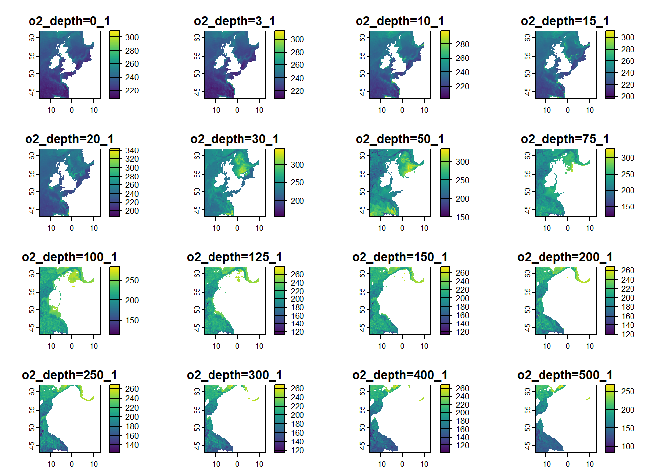
date <-as.POSIXct("2023-09-07", tz="UTC")subset_raster <- DO_raster[[terra::time(DO_raster)==date]] plot(subset_raster)
As you can see, the names of the layer follows this format variable_depth_numbering. The first part is the variable name. The middle part is the depth level in meters. The last part corresponds to the the order of the layers based on the time step, in this case daily. Layers with similar time-step have the same numbering. To extract the seafloor values, the raster can be divided into separate daily rasters and convert them into a tabular data as shown in the codes below.
library(dplyr)library(tidyr)library(stringr)library(kableExtra)time <-unique(terra::time(subset_raster)) # get timestampextent <- terra::ext(subset_raster) # get extent of the rasterx <- terra::as.data.frame(subset_raster, xy =TRUE, na.rm=FALSE) # convert raster into a dataframe, values in each depth are separated in columns
x
y
o2_depth=0_1
o2_depth=3_1
o2_depth=10_1
o2_depth=15_1
o2_depth=20_1
o2_depth=30_1
o2_depth=50_1
o2_depth=75_1
o2_depth=100_1
o2_depth=125_1
o2_depth=150_1
o2_depth=200_1
o2_depth=250_1
o2_depth=300_1
o2_depth=400_1
o2_depth=500_1
o2_depth=600_1
o2_depth=750_1
o2_depth=1000_1
-14.88894
61.93443
247.79
247.82
247.83
247.66
247.33
246.90
232.25
205.30
200.62
198.27
201.07
203.29
202.82
200.23
197.48
193.45
189.51
184.04
178.62
-14.77783
61.93443
245.95
245.97
245.96
245.83
245.59
245.16
230.79
201.87
195.80
196.08
198.95
204.13
203.53
202.49
200.40
201.73
191.59
183.50
171.19
-14.66672
61.93443
246.64
246.67
246.71
246.70
246.68
246.30
224.00
192.92
191.72
191.84
193.77
201.97
203.19
201.83
201.71
203.68
193.39
183.03
165.03
-14.55561
61.93443
246.67
246.70
246.72
246.70
246.68
246.40
234.41
213.42
201.61
202.78
205.50
210.09
209.73
209.88
209.66
208.28
202.76
192.44
176.61
-14.44450
61.93443
245.66
245.68
245.69
245.67
245.63
245.54
230.98
216.54
214.81
217.22
218.28
219.88
218.29
216.67
214.30
212.17
209.00
198.67
178.64
-14.33339
61.93443
245.11
245.13
245.14
245.11
245.03
245.01
230.77
213.56
213.74
215.08
215.99
218.44
219.34
219.59
218.88
217.78
214.43
198.26
181.08
depth_levels <- x %>%# get names of the columns that has depthselect(-any_of(c("x","X","y","Y"))) %>%colnames()x <- x %>% dplyr::filter(dplyr::if_any(.cols =!!depth_levels,.fns =~!is.na(.x))) %>%# remove rows that have NAs across depth levels (i.e., these are cells that are on land) dplyr::rename_with(., ~ stringr::str_extract(.x,"(?<=_depth=)[^_]+"), tidyselect::contains("_depth")) # rename the depth columns with just numbers
x
y
0
3
10
15
20
30
50
75
100
125
150
200
250
300
400
500
600
750
1000
-14.88894
61.93443
247.79
247.82
247.83
247.66
247.33
246.90
232.25
205.30
200.62
198.27
201.07
203.29
202.82
200.23
197.48
193.45
189.51
184.04
178.62
-14.77783
61.93443
245.95
245.97
245.96
245.83
245.59
245.16
230.79
201.87
195.80
196.08
198.95
204.13
203.53
202.49
200.40
201.73
191.59
183.50
171.19
-14.66672
61.93443
246.64
246.67
246.71
246.70
246.68
246.30
224.00
192.92
191.72
191.84
193.77
201.97
203.19
201.83
201.71
203.68
193.39
183.03
165.03
-14.55561
61.93443
246.67
246.70
246.72
246.70
246.68
246.40
234.41
213.42
201.61
202.78
205.50
210.09
209.73
209.88
209.66
208.28
202.76
192.44
176.61
-14.44450
61.93443
245.66
245.68
245.69
245.67
245.63
245.54
230.98
216.54
214.81
217.22
218.28
219.88
218.29
216.67
214.30
212.17
209.00
198.67
178.64
-14.33339
61.93443
245.11
245.13
245.14
245.11
245.03
245.01
230.77
213.56
213.74
215.08
215.99
218.44
219.34
219.59
218.88
217.78
214.43
198.26
181.08
x <- x %>% tidyr::pivot_longer(cols =-c(x,y), # pivot into long format, all parameter values in one column names_to ="depth",values_to ="z")
x
y
depth
z
-14.88894
61.93443
0
247.79
-14.88894
61.93443
3
247.82
-14.88894
61.93443
10
247.83
-14.88894
61.93443
15
247.66
-14.88894
61.93443
20
247.33
-14.88894
61.93443
30
246.90
x <- x %>% dplyr::mutate(depth =as.numeric(depth)) %>% dplyr::group_by(x,y) %>%# group by grid cell tidyr::drop_na() %>%# remove NAs dplyr::arrange(desc(depth), .by_group=TRUE) %>%# arrange depth from deepest to shallowest dplyr::slice_head() %>%# only extract the row with the deepest level dplyr::select(-depth)
x
y
z
-14.88894
43.00015
111.25
-14.88894
43.06682
118.13
-14.88894
43.13349
121.47
-14.88894
43.20016
117.86
-14.88894
43.26683
119.71
-14.88894
43.33350
115.99
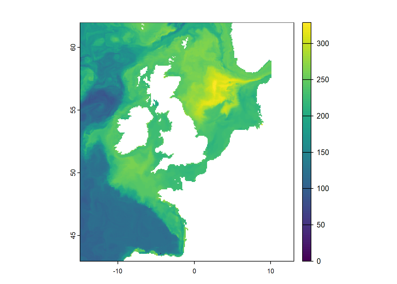
x <- terra::rast(x, type="xyz", crs="epsg:4326") # convert xyz dataframe into a SpatRaster objectterra::time(x) <- time # label the DateTime based from the original SpatRasternames(x) <- timex <- terra::extend(x,extent) # extend extent based on the original SpatRasterplot(x)
Now, we can bind all functions above into one and apply this to the downloaded NetCDF files.
ValueAtDeepest <-function(x){ # x is a SpatRaster object (several depth levels in each time step) time <-unique(terra::time(x)) # get unique time DateTime extent <- terra::ext(x) # get extent of the SpatRaster x = terra::as.data.frame(x, xy =TRUE, na.rm=FALSE) # convert SpatRaster into a data frame, values in each depth are separated in columns depth_levels <- x %>%# get names of the columns that has depthselect(-any_of(c("x","X","y","Y"))) %>%colnames() x <- x %>% dplyr::filter(dplyr::if_any(.cols =!!depth_levels,.fns =~!is.na(.x))) %>%# remove rows that have NAs across depth levels dplyr::rename_with(., ~ stringr::str_extract(.x,"(?<=_depth=)[^_]+"), tidyselect::contains("_depth")) %>% tidyr::pivot_longer(cols =-c(x,y), # pivot into long format, all parameter values in one column names_to ="depth",values_to ="z") %>% dplyr::mutate(depth =as.numeric(depth))gc() x <- x %>% dplyr::group_by(x,y) %>%# group by grid cell tidyr::drop_na() %>%# remove NAs dplyr::arrange(desc(depth), .by_group=TRUE) %>%# arrange depth from deepest to shallowest dplyr::slice_head() %>%# only extract the row with the deepest level dplyr::select(-depth) x <- terra::rast(x, type="xyz", crs="epsg:4326") # convert xyz dataframe into a SpatRaster object terra::time(x) <- time # label the DateTime based from the original SpatRasternames(x) <- time x <- terra::extend(x,extent) # extend extent based on the original SpatRasterreturn(x)}
The function above works on individual time-steps, putting it inside a for loop will take longer because this process is sequential. You can use parallel processing instead to speed up the processing. Since we have data spanning from 2006 to 2024, a nested loop was created with the outer for loop working through different NetCDF files and the inner for loop breaking down the task on a yearly basis. The parallel processing is implemented using foreach and it is nested within the inner for loop. Also, the function is created within the foreach function instead of creating it outside of the loops because sometimes the objects in the Global Environment are not transferred into the individual parallel workers.
library(terra)library(lubridate)library(doParallel)library(foreach)folder <-c("Salinity","Oxygen","pH") # specify the folder namesfor(i in1:length(folder)){ # outer loop working through each folder start <-Sys.time() # time tracking is used to get an overview on the processing time of each NetCDF file path <-unlist(list.files(path =paste0("./Data/Raw/Parameters/",folder[i]), # extract the path of the NetCDF filespattern='.nc$', all.files=TRUE, full.names=TRUE)) raster <-rast(path) # import NetCDF as SpatRaster year <-as.character(terra::time(raster)) %>%substr(.,1,4) %>%unique() rastList <-vector(mode="list", length=length(year)) # create a list that will contain yearly processed rasters for(j in1:length(year)){ # inner loop that processes the raster each yearcat(sprintf("\033[33;1m%-1s\033[0m %-12s \033[33mExtracting seafloor values from\033[0m\033[36;1m %-s %-s \033[0m\033[33mfile...\033[0m\r","i","[Processing]",basename(path),year[j])) date_min =ymd(paste0(year[j],"0101"), tz="UTC") date_max =ymd(paste0(year[j],"1231"), tz="UTC") dateRange <-seq(date_min,date_max, by ="day") # generate a range of dates because foreach works on a daily time step dates <-unique(terra::time(raster[[terra::time(raster) %in% dateRange]])) # this vector is created because sometimes the NetCDF files contains missing dates varname <-paste0("bottom_",unique(varnames(raster))) # specify variable name to be used in writing the processed NetCDF file longname <-paste0("Seafloor ",tolower(unique(longnames(raster)))) # specify long variable name to be used in writing the processed NetCDF file unit <-unique(units(raster)) # specify variable unit to be used in writing the processed NetCDF file n_cores <-8# specify the number of parallel workers, use to cl <-makeCluster(n_cores)registerDoParallel(cl) processed <-foreach(k =1:length(dates), .export=c("path"), .packages =c("terra","Rcpp","dplyr","stringr","tidyr","tidyselect")) %dopar% { ValueAtDeepest <-function(x){ time <-unique(terra::time(x)) extent <- terra::ext(x) x = terra::as.data.frame(x, xy =TRUE, na.rm=FALSE) depth_levels <- x %>%select(-any_of(c("x","X","y","Y"))) %>%colnames() x <- x %>% dplyr::filter(dplyr::if_any(.cols =!!depth_levels,.fns =~!is.na(.x))) %>% dplyr::rename_with(., ~ stringr::str_extract(.x,"(?<=_depth=)[^_]+"), tidyselect::contains("_depth")) %>% tidyr::pivot_longer(cols =-c(x,y), names_to ="depth",values_to ="z") %>% dplyr::mutate(depth =as.numeric(depth))gc() x <- x %>% dplyr::group_by(x,y) %>% tidyr::drop_na() %>% dplyr::arrange(desc(depth), .by_group=TRUE) %>% dplyr::slice_head() %>% dplyr::select(-depth) x <- terra::rast(x, type="xyz", crs="epsg:4326") terra::time(x) <- time names(x) <- time x <- terra::extend(x,extent) return(x) } raster <-rast(path) subRaster <- raster[[terra::time(raster)==dates[k]]] # subset raster per day bottom_values <-ValueAtDeepest(subRaster) %>%# apply the custom function terra::focal(x = ., w =3, fun="mean", na.policy="only", na.rm=TRUE) %>%# calculate "moving window" values to fill gaps near the coast terra::wrap() # pack processed SpatRaster so it can be imported back to the Global Environmentreturn(bottom_values) }stopCluster(cl) # stop parallel backend processed <-lapply(processed,unwrap) # unwrap packaged SpatRaster in the Global Environment rastList[[j]] <-rast(processed) # append SpatRaster into a list } final_raster <-rast(rastList) # convert list of SpatRasters into one SpatRaster object terra::writeCDF(final_raster, # write processed SpatRaster into NetCDF fileoverwrite =TRUE,varname = varname,longname = longname,unit = unit,filename =paste0("./Data/Processed/Parameters/processed_",basename(path))) end <-Sys.time() timeDiff <-round(difftime(end,start, units="hours"), digits=4)cat(sprintf("\033[32;1m%-1s\033[0m %-12s %-s seafloor values extracted. Elapsed time is %-s hours. \033[0m\n","✔","[Completed]",basename(path),timeDiff)) # print processing updatefile.remove(path) # delete raw file to save storage space}