Data Exploration
Once your data is ready for model training, it is always a good practice to perform data exploration to remove possible outliers and colinear predictors or check conformity of the data distribution to the assumptions of the chosen modelling algorithm. Zuur et al. 2010 has comprehensively described a protocol in data exploration. In this section, we will show some R codes to perform data exploration on binary response variable with continuous predictor variables.
Data Splitting
Before you perform data exploration, you need to split first the dataset into training and test sets. Data exploration is part of the model training process. Hence, it should only be done on the training data. The test data should be held out at the start to prevent information leakage. It is meant to provide unbiased evaluation of the model performance. Our dataset contains spatial and temporal structure and we want the model to perform forecasting. So, we will test the model performance in three aspects:
test_time - accuracy on data points outside of the temporal range but within the spatial range of the training set
test_location - accuracy on data points outside of the spatial range but within the temporal range of the training set
test_loc_time - accuracy on data points outside of the spatial and temporal range of the training set
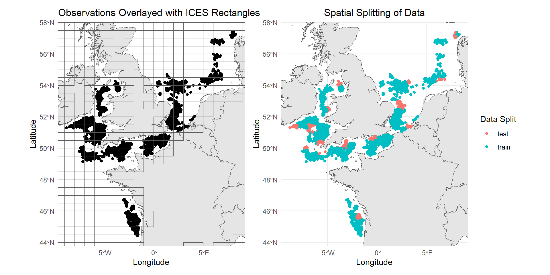
To split the data, we need to assign the data points into spatial and temporal blocks. The map below shows the spatial range of the dataset. You can use any predefined polygons to group the data points into spatial blocks. Here, we will be using the ICES statistical rectangles. You can download the shapefile in the interactive map viewer from ICES. Based on visual inspection, the observations appear to form clusters. To create the test dataset, one ICES rectangle is selected from each cluster. This approach avoids holding out an entire cluster (e.g., all data points from the Bay of Biscay), which could exclude region-specific predictor patterns, such as unique temperature ranges. Such exclusions might cause the model to struggle with generalizing across the broader spatial range of observations.
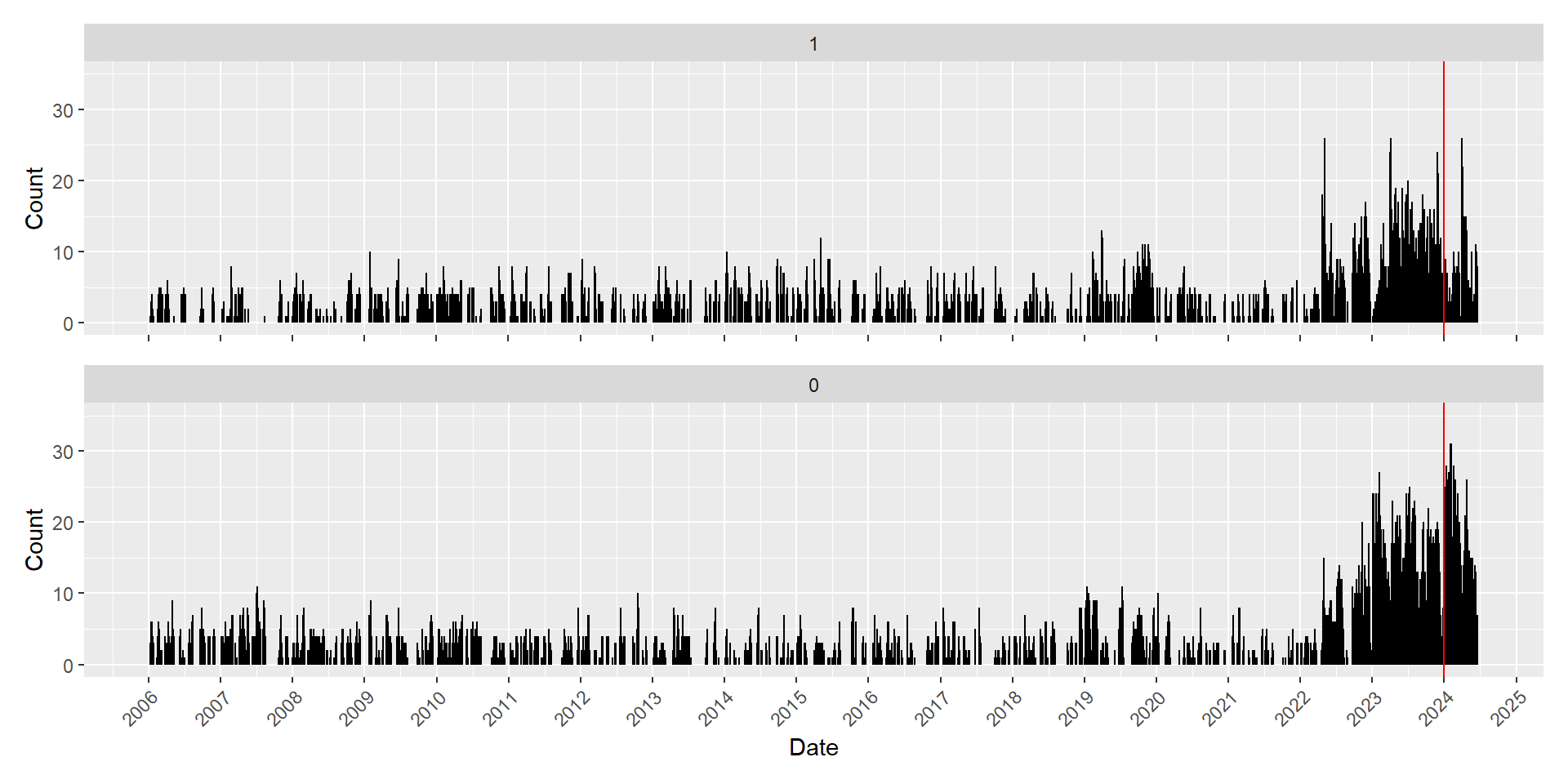
The catch data ranges from 2006 until mid 2024, where most data are concentrated between 2022 to 2024. To split the data in time, all data points from 2006-01-01 to 2023-12-31 will be assigned to the training set while data points after 2023-12-31 will be used for testing model performance.
With specifications we have set above, we can now properly split the dataset into 4 sets - 1 training and 3 sets for testing. First, the data points need to be converted to an sf object and assign them to spatial blocks through spatial intersection with the ICES Rectangles polygon. Then, use the specified date above as a cut off for splitting the data in time.
library(tidyverse)
library(sf)

df <- read.csv("./Data/Catch/catch_with_predictors.csv") %>%
  mutate(Date = as.Date(Date),                                                  # convert to class Date for plotting
         Year = as.numeric(substring(Date,1,4)))                                # create Year column for creating facets in the plot

land <- st_read("./Data/Polygons/land.shp", quiet=TRUE)                         # read vector data on land
ICES <- st_read("./Data/Polygons/ICES_rectangles.shp", quiet=TRUE)              # read vector data on ICES rectangles

df <- df %>%
  mutate(x = Longitude,
         y = Latitude) %>%
  st_as_sf(coords=c("x","y"), crs=st_crs(4326))                                 # convert dataframe to sf object

df <- df %>%
  st_join(., ICES, join=st_intersects)                                          # spatial join through intersection between catch data and ICES rectangles

test_blocks <- c("20E8","28E4","29E2","29E4","29E6","30E9","31E1","31E3","31F3",# selected ICES rectangles as spatial blocks for test set
                 "33E5","34E5","34F2","37E6","37F3","37F6","43F7")

df <- df %>%
  mutate(data_split =
           case_when(ICESNAME %in% test_blocks &                                # classify data points to different data split sets
                       Date>as.Date("2023-12-31")     ~ "test_loc_time",
                     ICESNAME %in% test_blocks &
                       Date<=as.Date("2023-12-31")    ~ "test_location",
                     !(ICESNAME %in% test_blocks) &
                       Date>as.Date("2023-12-31")     ~ "test_time",
                     !(ICESNAME %in% test_blocks) &
                       Date<=as.Date("2023-12-31")    ~ "train",
                                               TRUE   ~ "remove"
                     )) %>%
  st_set_geometry(., NULL)                                                      # convert sf back to dataframe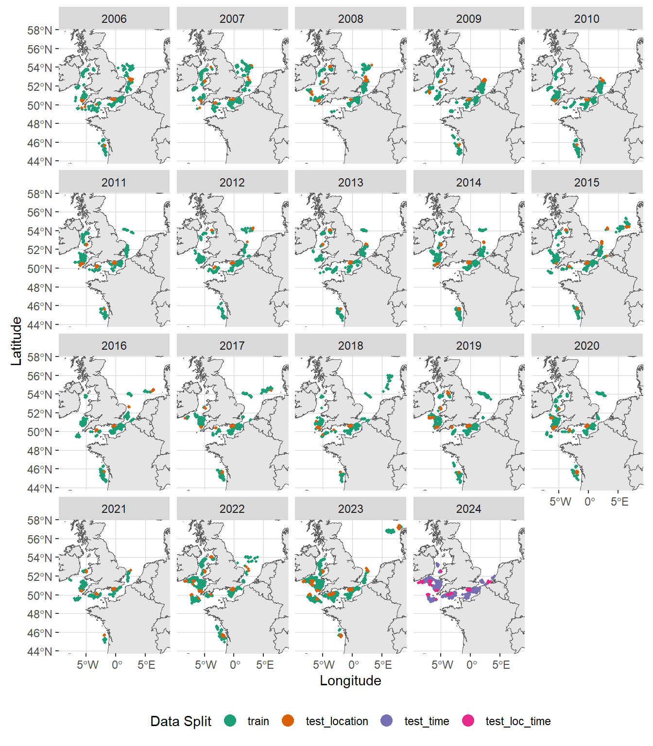
As shown in the plot above, the training data points (in green) span the period from 2006 to 2023. Data points within this time frame but located outside the training locations (in orange) will be used to evaluate the model’s spatial extrapolation accuracy. Data points from 2024 will be used to assess temporal prediction performance (in violet) and spatio-temporal extrapolation capabilities (in pink).
Create New Predictors
In the previous section, we incorporated environmental data from CMEMS and their lagged values into the catch data. These lagged predictors are often highly collinear, particularly for variables that do not exhibit significant daily variation. Despite this, we aim to investigate whether past values of a predictor influence the response variable. To address the issue of collinearity, we created a proxy for lags by calculating the change in values over time. Specifically, we used the difference between the current value and its lagged value, as illustrated in the code below. These derived features are denoted by the prefix delta, followed by the lag number (in days). We can also create dummy variables for time both to represent seasonality ordinalDay (Line 4) and long-term temporal trend time_trend (Line 5). The time_trend is a numeric variable which is calculated by taking the time difference (in seconds) between the Date in each observation and the earliest recorded Date in the data set. Since this calculation yields a huge number for recent Dates and this might be problematic during model training, the computed values are divided by 1e9.
library(lubridate)

df <- df %>%
  mutate(ordinalDay = yday(Date),
         time_trend = as.numeric(Date - min(df$Date))/1e9,
         Year = year(Date),
         Catch = factor(Catch, levels=c(1,0)),
         current = sqrt(current_u^2 + current_v^2),
         lag1_current = sqrt(lag1_current_u^2 + lag1_current_v^2),
         lag2_current = sqrt(lag2_current_u^2 + lag2_current_v^2),
         delta1_ssh = ssh - lag1_ssh,
         delta2_ssh = ssh - lag2_ssh,
         delta1_wave_mean = wave_mean - lag1_wave_mean,
         delta2_wave_mean = wave_mean - lag2_wave_mean,
         delta1_current = current - lag1_current,
         delta2_current = current - lag2_current,
         delta1_current_u = current_u - lag1_current_u,
         delta2_current_u = current_u - lag2_current_u,
         delta1_current_v = current_v - lag1_current_v,
         delta2_current_v = current_v - lag2_current_v,
         delta7_DO = DO - lag7_DO,
         delta14_DO = DO - lag14_DO,
         delta7_pH = pH - lag7_pH,
         delta14_pH = pH - lag14_pH,
         delta60_pp = pp - lag30_pp,
         delta60_pp = pp - lag60_pp,
         delta7_salinity = salinity - lag7_salinity,
         delta14_salinity = salinity - lag14_salinity,
         delta7_bottomT = bottomT -lag7_bottomT,
         delta14_bottomT = bottomT - lag14_bottomT) %>%
  select(ID,Date,Species,Catch,ordinalDay,Year,time_trend,Longitude,Latitude,
         depth,ssh,wave_mean,current,current_u,current_v,
         DO,pH,pp,salinity,bottomT,
         contains("delta"))
Check Class Frequency
Now that we have splitted the data into train and test sets, let’s check the frequency of each class (presence and absence of Catch) in each data split set. It is important to do this because this dictates the training strategy and the type of metrics to use in evaluating the model performance. As you can see from the tibble below, there are more absences than presences in the dataset. Strategies to mitigate this class imbalance will be discussed in the next section on Machine Learning.
df %>%
  group_by(data_split,Catch) %>%
  summarise(n())
# A tibble: 8 × 3
# Groups: data_split [4]
data_split Catch `n()`
<chr> <fct> <int>
1 test_loc_time 1 69
2 test_loc_time 0 352
3 test_location 1 772
4 test_location 0 894
5 test_time 1 635
6 test_time 0 1980
7 train 1 9131
8 train 0 10763Check for Outliers in the Predictors
There are different ways to check for outliers and one classical tool is the boxplot as shown below left. The box represents the spread of the central 50% of the data and where the median is indicated by the central line. The lines that extends from the box represent the remaining data and the points are possible outliers.Another visual tool mentioned by Zuur et al. 2010 to detect outliers is the Cleveland plot (shown below right). This visualization plots the predictor values against the row index of the observation. Since our data has a temporal structure, we can plot the predictor of interest against time. The Cleveland plot can help you to discern whether the outliers shown by the boxplot are actual outliers.
📣 Note: We will be using XGBoost in training our model. This algorithm is not sensitive to outliers so we are keeping the outliers for this exercise.
library(patchwork)

train_data <- filter(df, data_split=="train")

boxplot <- train_data %>%
  ggplot(aes(x=Catch, y=bottomT, color=Catch)) +
    geom_boxplot() +
    theme_minimal()

cleveland <- train_data %>%
  ggplot(aes(x=Date, y=bottomT, color=Catch)) +
    geom_point(size=0.8)  +
    scale_x_date(date_breaks="2 years", date_label="%Y") +
    guides(color = guide_legend(override.aes = list(size = 4))) +
    theme_minimal()

boxplot + cleveland +
  plot_layout(widths = c(1, 4))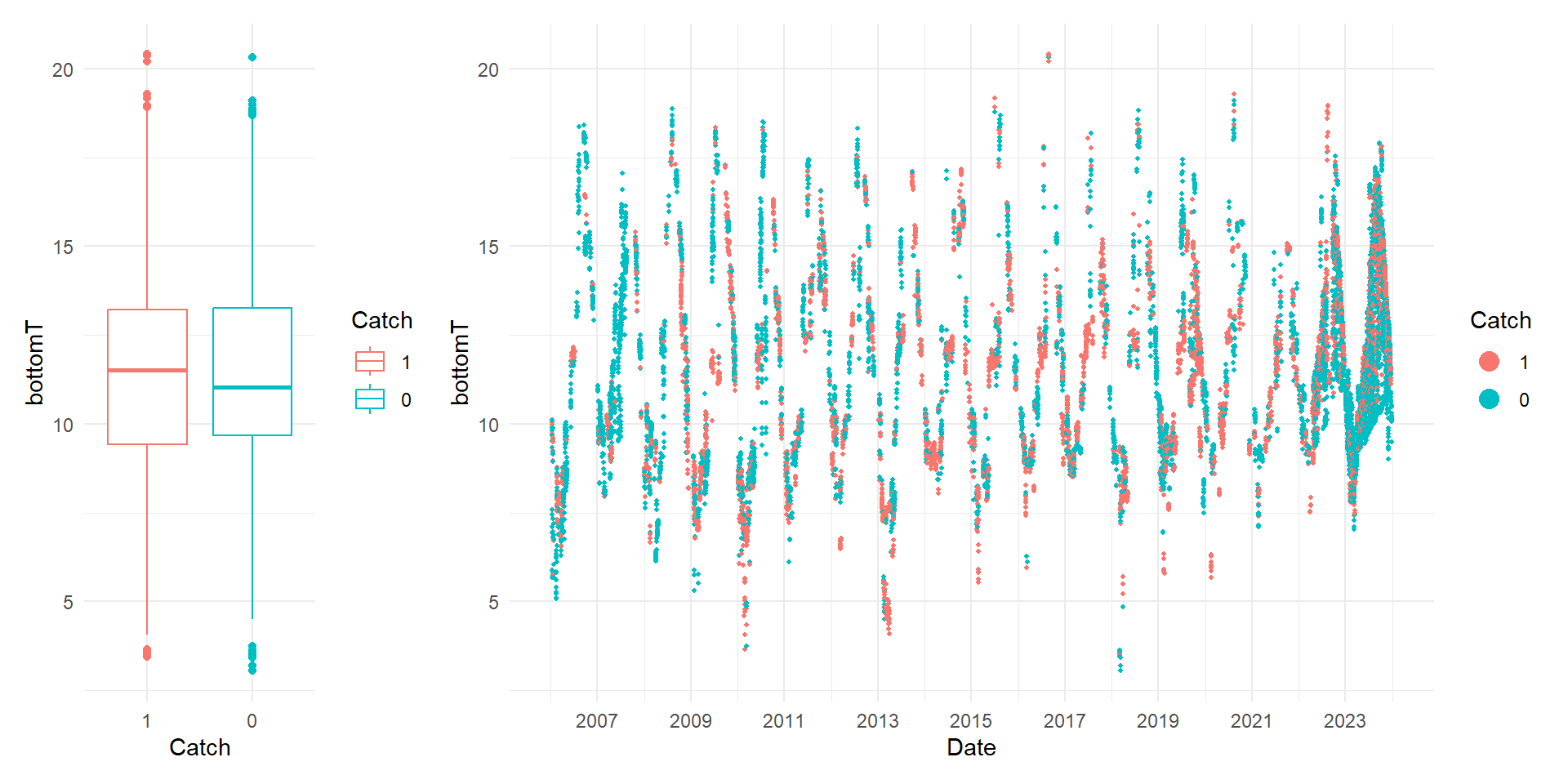
Check for Collinearities in the Predictors
We selected predictors based on environmental factors that may influence the biology of the target fish species, as well as sea state variables that could impact their catchability. However, some of these predictors may be collinear, which could pose challenges during model training. While it is generally unnecessary to remove collinear predictors when using algorithms like Random Forests or XGBoost, addressing collinearity can still offer benefits. These include improved model interpretability, enhanced computational efficiency, and potentially better overall performance. We can use an interactive correlation plots to check the pairwise correlations of the predictors.
library(plotly)
library(corrr)

vars <- train_data %>%
    select(Year:delta14_bottomT) %>%
    colnames()

cor_matrix <- train_data %>%
  select(all_of(vars)) %>%
  correlate(method = "spearman") %>%
  shave() %>%
  rplot(print_cor = TRUE) +
    theme(axis.text.x = element_text(angle = 45, hjust = 1),
          plot.title = element_text(hjust = 0.5, size = 18))

ggplotly(cor_matrix)
Based on the correlation values plotted above, some predictors have high pairwise correlation values. There is no consensus on the threshold value for removing collinear predictors, but any value larger than 0.8 is generally accepted as very high correlation. We will remove one predictor in each pair of collinear predictors that satisfies this criteria.
train_data <- train_data %>%
  select(-Year,-delta7_DO,-delta7_bottomT)
Cross-Validation
In Machine Learning (ML), certain parameters must be defined before training a model; these are known as hyperparameters. Unlike other model parameters, hyperparameters are not estimated by the ML algorithm, so it is up to the modeller to determine their optimal values. This process is typically done through a grid search, where the model is trained using different combinations of hyperparameters, and the best set is selected based on performance. To evaluate model performance, the training data can be split into subsets, using one portion to train the model and the remainder to validate it.
📣 Remember: Never use the test data during the training process and only use it during the final evaluation of the model.
We can perform this sampling technique multiple times and obtain a mean value for model performance. This strategy of repeated sampling to estimate the performance of a predictive ML model is called cross-validation (CV). In the field of spatial modelling, there is no consensus as to which type of cross-validation to use. There are two conflicting CV methods. The first approach involves using spatial (and temporal) cross-validation, which partitions the data into folds. In this method, the holdout dataset is selected to lie outside the spatial (temporal) range of the training dataset. This approach is based on the argument that the data follows a spatial (temporal) structure. Traditional random cross-validation ignores spatial (temporal) autocorrelation and can result in overly optimistic accuracy estimates because training and test data points may be located close to each other in space (and time), leading to artificially high performance metrics (Roberts et al. 2017, Valavi et al. 2018, Meyer et al. 2019) . However, Wadoux et al. 2021 argues that this strategy doesn’t have theoretical basis and produces overly pessimistic model performance. Probability sampling such as simple random sampling should be used in evaluating the model accuracy. Choosing which strategy influences the outcome of a fitted model (Huang et al. 2024). Hence, we will test both CV methods and check which one will produce the most accurate model.
Space-Time Cross-Validation
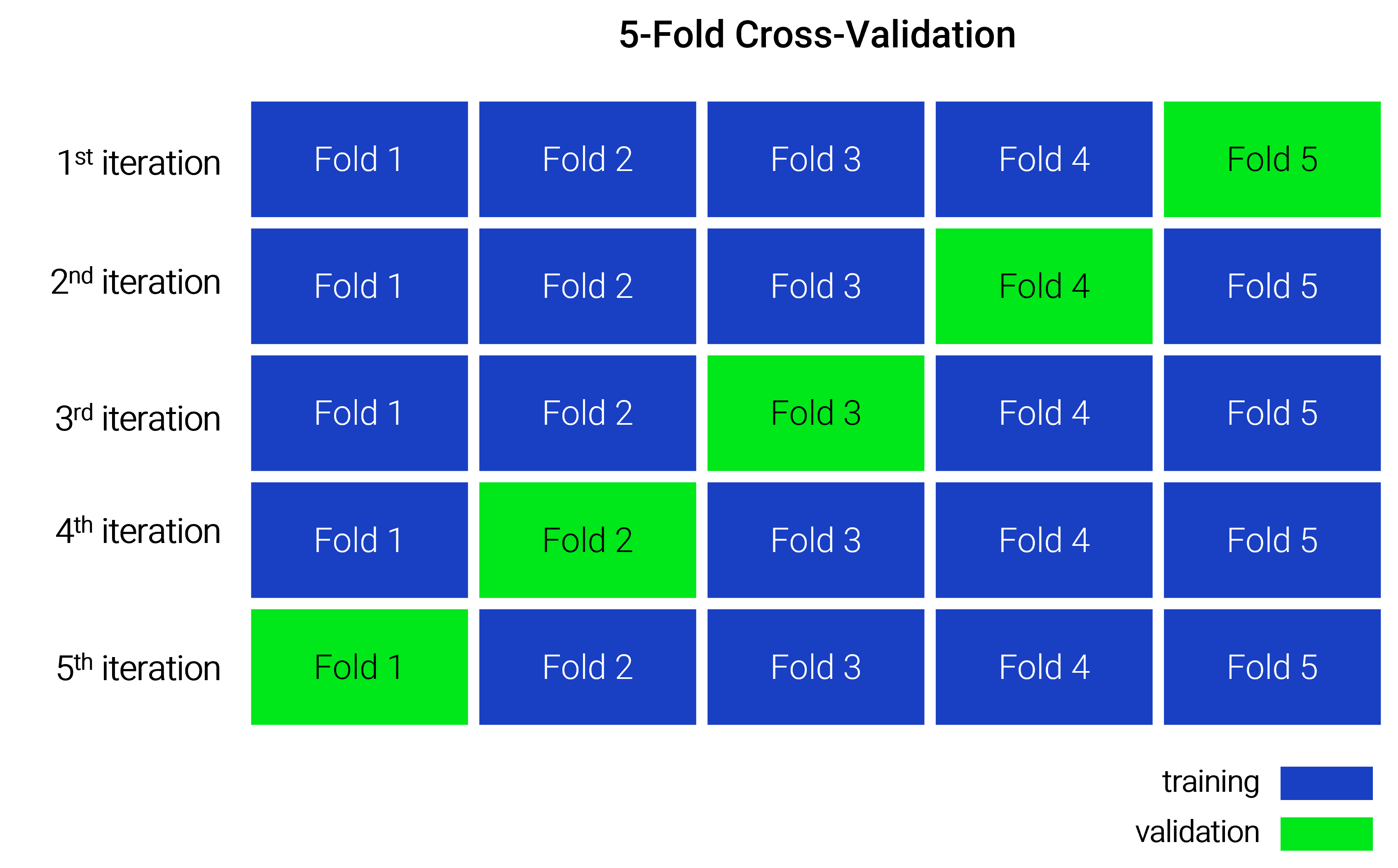
This CV method is a specialized form of k-fold cross-validation, where data is partitioned into subsets (called folds) with consideration for spatial and temporal blocking. These folds are then used for training and validation, as illustrated in the figure below. The folds are mutually exclusive, meaning that each data point appears in the validation set only once.
In this CV method, we will be assigning the data points into spatial and temporal blocks. In the first subsection, we have already assigned the data points into spatial blocks (i.e., ICES Statistical Rectangles) as shown in the plot below.
Code
palette <- sample(scales::hue_pal()(length(unique(train_data$ICESNAME))))

ggplot() +
  geom_sf(data=land) +
  geom_point(data=train_data, aes(x=Longitude, y=Latitude, color=ICESNAME),size=0.03) +
  scale_color_manual(values = palette) +
  ggtitle("Spatial Folds") +
  xlim(min(train_data$Longitude)-1,max(train_data$Longitude)+1) +
  ylim(min(train_data$Latitude)-1,max(train_data$Latitude)+1) +
  theme(plot.title = element_text(hjust = 0.5, size = 18),
        legend.position = "none")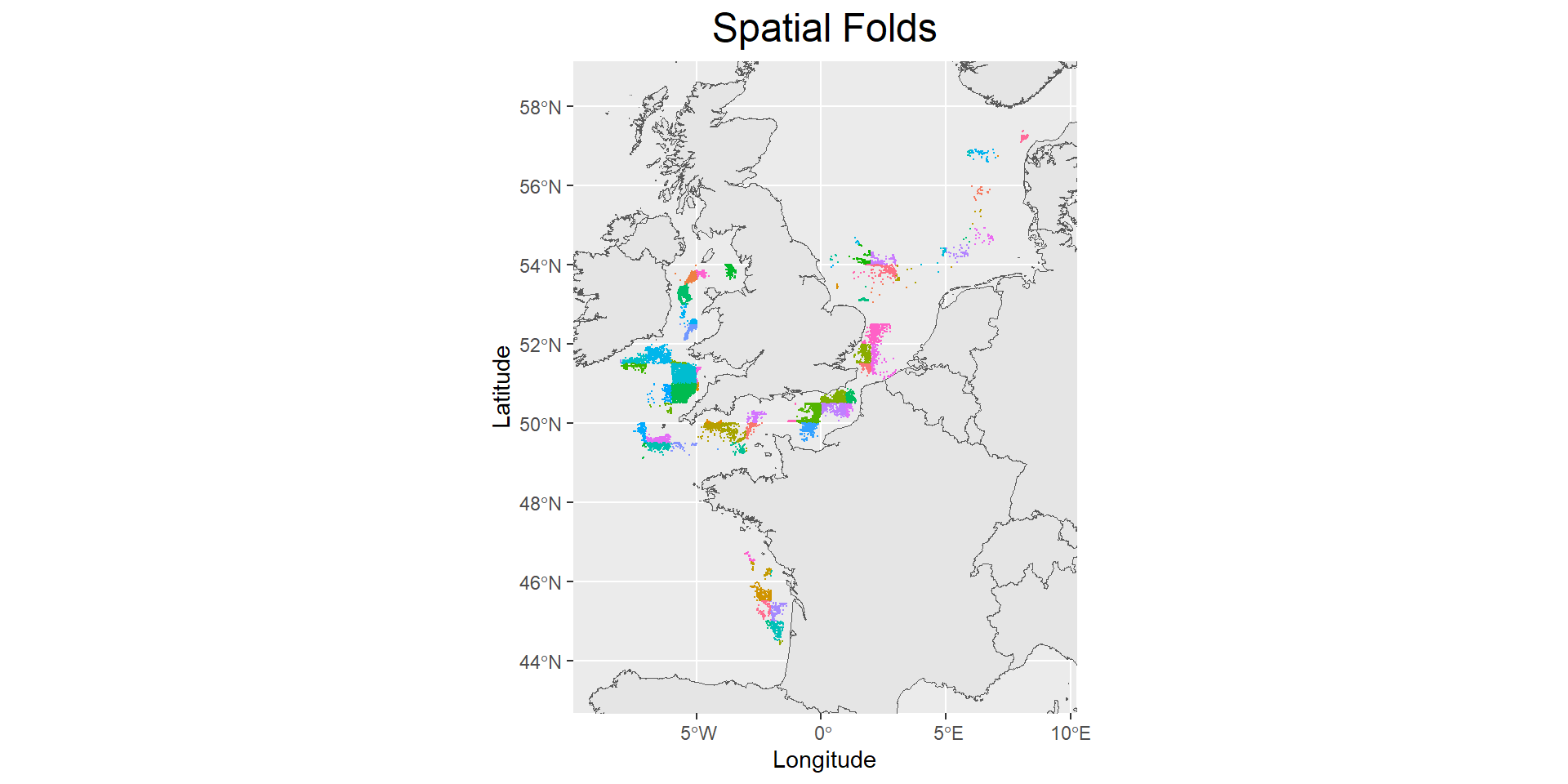
The combination of Year and Month will serve as unique temporal blocks. The CAST package will be used to assign data points into space-time cross-validation (CV) folds, after which the caret package will create the CV object. For fitting Machine Learning models, we will use tidymodels, a suite of packages designed for modeling and machine learning based on tidyverse principles. As a result, the caret CV object must be converted into a tidymodels CV object using the rsample package.
library(CAST)
library(caret)
library(rsample)

train_data <- train_data %>%
  mutate(year_month = substring(Date,1,7))

folds <-  train_data%>%                                  # create temporal blocks
  CreateSpacetimeFolds(spacevar="ICESNAME",                                     # large list containing the row index of observations per folds
                       timevar="year_month",
                       k=10,                                                    # number of folds
                       seed = 789)

train_index <- folds$index                                                      # row indexes for training data points
names(train_index) <- c("Fold1","Fold2","Fold3","Fold4","Fold5",                # rename folds
                  "Fold6","Fold7","Fold8","Fold9","Fold10")

train_indexOut <- folds$indexOut                                                # row indexes for test data points
names(train_indexOut) <- c("Fold1","Fold2","Fold3","Fold4","Fold5",
                     "Fold6","Fold7","Fold8","Fold9","Fold10")

SpaceTime_CV <- caret::trainControl(method = "cv",                              # create caret CV object
                                    number = 10,
                                    index = train_index,
                                    indexOut = train_indexOut)

SpaceTime_CV <- caret2rsample(SpaceTime_CV,train_data)                          # convert to rsample CV object
Let’s examine the count of 1s and 0s in the training and validation sets for each fold. In the plot below, each facet represents an individual fold, with the bar labels indicating the actual counts. As shown, there is a class imbalance present in both the training and validation sets. To address this, mitigation techniques should be applied during model training to ensure the model can effectively learn the target class (Catch = 1). Additionally, an appropriate evaluation metric must be selected to account for the class imbalance in the validation set.
Code
summary_tbl <- tibble()

for(i in 1:nrow(SpaceTime_CV)){

  train <- analysis(get_rsplit(SpaceTime_CV,index=i)) %>% mutate(split = "train")
  test <- assessment(get_rsplit(SpaceTime_CV,index=i)) %>% mutate(split = "validation")

  summary_tbl <- bind_rows(train,test) %>%
    group_by(split,Catch) %>%
    summarise(count = n()) %>%
    mutate(proportion_count = (count / sum(count)),
           fold = i) %>%
    bind_rows(summary_tbl,.)
}

plot <- ggplot(summary_tbl, aes(x = split, y=proportion_count,fill = Catch)) +
  geom_bar(stat = "identity",position = "fill") +
  facet_wrap(~fold, nrow=2) +
  geom_text(aes(label = count), size = 2,
            position = position_fill(vjust = 0.5))

ggplotly(plot)
Monte-Carlo Cross-Validation
Unlike the cross-validation method described earlier, this approach does not involve creating data folds. Instead, it uses repeated simple random sampling (without replacement) to split the training data into training and validation sets. As a result, a data point may appear in the validation set of multiple CV groups or may not be included at all. Refer to the figure below for a comparison between k-fold CV and Monte Carlo CV.

To create Monte Carlo cross-validation groups, we can use the mc_cv() function from the rsample package.
MonteCarlo_CV <- rsample::mc_cv(train_data,
                                prop = 3/4,      # proportion of data to be retained for modeling
                                strata = Catch,  # to make sure the frequency of 1s and 0s are equal in both training and validation sets
                                times = 10)      # number of times to repeat the sampling
Let’s also examine the counts of 1s and 0s in each dataset. As shown, the frequency of each level of Catch is consistent between the training and validation sets across all folds. However, a slight class imbalance is still present in each set.
Code
summary_tbl <- tibble()

for(i in 1:nrow(MonteCarlo_CV)){

  train <- analysis(get_rsplit(MonteCarlo_CV,index=i)) %>% mutate(split = "train")
  test <- assessment(get_rsplit(MonteCarlo_CV,index=i)) %>% mutate(split = "validation")

  summary_tbl <- bind_rows(train,test) %>%
    group_by(split,Catch) %>%
    summarise(count = n()) %>%
    mutate(proportion_count = (count / sum(count)),
           fold = i) %>%
    bind_rows(summary_tbl,.)
}

plot <- ggplot(summary_tbl, aes(x = split, y=proportion_count,fill = Catch)) +
  geom_bar(stat = "identity",position = "fill") +
  facet_wrap(~fold, nrow=2) +
  geom_text(aes(label = count), size = 2,
            position = position_fill(vjust = 0.5))

ggplotly(plot)