The goal of building the fishing suitability model is to generate highly accurate predictions. To achieve this, we will leverage various techniques in Machine Learning (ML) to construct our predictive model. While there are numerous ML algorithms, each with its own strengths and limitations, we will focus on demonstrating the model-building process using Random Forest as an example.
Basics of tidymodels
Implementing machine learning in R is now easier with the development of the package tidymodels. It is not one single package like caret but an ecosystem of modular packages. Just like caret, it acts as a wrapper of several ML packages making the implementation more straightforward and simplified. It embraces the “tidyverse” design philosophy, ensuring compatibility with other tidyverse packages like ggplot2 and dplyr.
Preprocessing
Data preprocessing is a critical first step in any Machine Learning (ML) workflow, as it transforms raw data into a format suitable for model training. Some preprocessing steps, such as outlier removal and the modification or creation of new predictors, have already been covered in the Data Exploration section. Here, we will focus on additional preprocessing steps tailored specifically to our dataset and the ML algorithm we intend to implement. These steps will be defined using the recipes package, which allows us to bundle preprocessing instructions with the training data and specify the roles of each variable within the dataset, creating a recipe object.
Before we proceed with creating a recipe, let’s make sure that the dataset doesn’t contain any unnecessary variables.
The code below demonstrates the creation of a recipe, with each step connected using the pipe operator %>%, following the tidyverse style of coding. The recipe() function (Line 5) initializes the recipe object, allowing you to define the input data and specify the roles of each variable in the model fitting process. This function only requires a template dataset, meaning you don’t need to supply the entire dataset. Instead, you can provide just the first few rows of the data. Additionally, the roles of the variables are defined by specifying a model formula.
📣 Note from the recipes package: No in-line functions should be used in the model formula (e.g. log(x), x:y, etc.) and minus signs are not allowed. These types of transformations should be enacted using step functions in this package. Dots are allowed as are simple multivariate outcome terms (i.e. no need for cbind; see Examples). A model formula may not be the best choice for high-dimensional data with many columns, because of problems with memory.
The left-hand side of the tilde ~ represents the response variable (e.g., Catch), while the right-hand side contains the explanatory variables (predictors). The . symbol refers to all remaining variables in the dataset. Feature engineering steps in the recipe are specified using functions prefixed with step_. For those unfamiliar with the term, feature engineering encompasses various data manipulation techniques such as variable transformations, creation of interaction terms, dummy coding, and imputation. A comprehensive list of step_ functions supported by the recipes package can be found here. These step_ functions can be applied to specific columns or to groups of columns sharing similar properties. Variables can be selected in two ways: using dplyr-like selection tools or recipes-specific functions. Detailed explanations of variable selection methods can be found here. The recipes-specific functions are listed here.
In Line 6, rows with NA values will be removed from the dataset. This operation is applied to all columns with assigned roles in the recipe. As specified earlier, Catch is designated as the response variable, while the remaining variables are predictors. In Line 7, predictors with zero or near-zero variance are removed. While this step is not strictly necessary for Random Forest, it can enhance the computational efficiency of model fitting by eliminating predictors that contribute minimal or no meaningful information to the decision tree splits. Each model type requires specific preprocessing steps. A table of recommended preprocessing per model type is shown in this webpage.
• Sparse, unbalanced variable filter on: all_predictors()
• SMOTE based on: Catch
• Variables removed: Latitude Longitude
To effectively predict suitable catches, the model should prioritize learning from the positive class. However, the dataset exhibits class imbalance, with significantly more negative (0) than positive (1) instances, as shown in the data exploration section. This imbalance can bias the training process towards the majority class, potentially hindering the model’s ability to accurately predict the rare positive cases. There are different strategies to mitigate this - apply case weights or upsample/downsample. We will be upsampling the minority positive class. If you’re interested to use case weights, you can refer to this blog by Max Kuhn. Here we will apply SMOTE from the themis package (Line 8). SMOTE stands for Synthetic Minority Oversampling Technique where it generates new instances of the minority class using nearest neighbors of these instances and not duplicating existing samples.
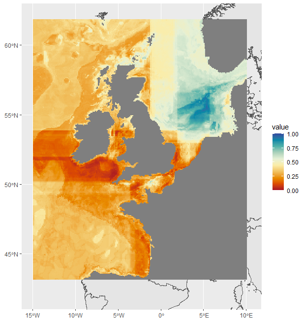
Lastly, we remove Latitude and Longitude from the dataset because it can create spatial artefacts in the prediction map as shown below. It has been noted that incorporating spatial coordinates in model training especially tree-based models are not suitable for clustered samples and can lead to spatial overfitting (Milà et. al, 2024). We did not remove these coordinates right in the beginning because we want SMOTE to consider the proximity of data in space and time in creating new instances.
📣 Note: The type of data preprocessing needed is different between models. For a list of recommended preprocessing steps, you can consult the table here.
Model Specification
To specify the ML algorithm we want to use, we will use the parsnip package. This package provides a unified interface for defining and fitting machine learning algorithms, streamlining the process across a variety of modeling engines (e.g., lm, randomForest, xgboost). You can check this link for the supported models by parsnip. By standardizing the modeling syntax and adopting consistent key parameter names across independent ML packages, parsnip enhances readability and usability. This is particularly beneficial for beginners, as it simplifies the often fragmented and inconsistent syntax found in different packages.
To specify a model using the parsnip package, only three functions are needed:
Model Type: Use the rand_forest() function to define a random forest model. Here, we also specify the hyperparameter values (referred to as tuning parameters in tidymodels). The random forest implementation in tidymodels supports three key hyperparameters:
mtry: The number of randomly selected predictors.
trees: The total number of trees in the forest.
min_n: The minimum number of samples required at a leaf node.
📣 Hyperparameters: Configuration settings external to the learning process that control the behavior of a machine learning model or training algorithm. Unlike model parameters, which are learned from the data during training (e.g., weights in a neural network), hyperparameters are set before training begins and can significantly influence model performance and training efficiency.
Engine: Specify the computational engine for the model using the set_engine() function. Tidymodels supports six engines for random forest. Engine-specific arguments can also be defined in this function. In the example below, we have included importance = "impurity" argument. This measures variable importance based on the total decrease in node impurity (e.g., Gini index for classification, residual sum of squares for regression) contributed by splits involving the variable.
Mode: Specify the type of modeling problem with the set_mode() function. This depends on the nature of the response variable in your dataset. Since our response variable Catch is binary, we will use "classification" as the mode.
By combining these three steps, you can fully define a random forest model tailored to your specific data and problem.
Random Forest Model Specification (classification)

Main Arguments:
  mtry = 10
  trees = 1000
  min_n = 5

Engine-Specific Arguments:
  importance = impurity

Computational engine: ranger
Binding the Model with Preprocessing
Now that we have specified both the preprocessing steps and the model specification, we can tie them together using the package workflows. This streamlines the modelling process and make sit easy to reuse on different datasets. To create a workflow, you only need to use the workflow() function and then add the parsnip and recipe objects.
══ Workflow ════════════════════════════════════════════════════════════════════
Preprocessor: Recipe
Model: rand_forest()

── Preprocessor ────────────────────────────────────────────────────────────────
4 Recipe Steps

• step_naomit()
• step_nzv()
• step_smote()
• step_rm()

── Model ───────────────────────────────────────────────────────────────────────
Random Forest Model Specification (classification)

Main Arguments:
  mtry = 10
  trees = 1000
  min_n = 5

Engine-Specific Arguments:
  importance = impurity

Computational engine: ranger
Resampling and Tuning
When creating the parsnip model, we initially assigned arbitrary values to the tuning parameters. However, there are numerous possible combinations of these values, and only a subset of these combinations will result in an optimally accurate predictive model. To identify the best combination, we can use the tune package to perform a search across unique sets of tuning parameter values. There are different strategies for hyperparameter tuning but we will be using grid search here. For a more in-depth understanding of hyperparameter tuning, please refer to this link.
First, we need to modify the tuning parameters in the parsnip model to tune() as shown in the codes below. Then, the workflow needs to be updated to reflect these changes.
══ Workflow ════════════════════════════════════════════════════════════════════
Preprocessor: Recipe
Model: rand_forest()

── Preprocessor ────────────────────────────────────────────────────────────────
4 Recipe Steps

• step_naomit()
• step_nzv()
• step_smote()
• step_rm()

── Model ───────────────────────────────────────────────────────────────────────
Random Forest Model Specification (classification)

Main Arguments:
  mtry = tune()
  trees = tune()
  min_n = tune()

Engine-Specific Arguments:
  importance = impurity

Computational engine: ranger
The second step is to create resamples, which allow us to evaluate the performance of different hyperparameter configurations on unseen data in a robust and unbiased manner. It is crucial to avoid using the test dataset during the training process to prevent data leakage and ensure a fair evaluation. Instead, resamples must be generated from the training data. In this case, we have already created resamples in the previous section on cross-validation, using both SpaceTime_CV and MonteCarlo_CV. These resampling strategies will be utilized to assess the model’s performance across various hyperparameter combinations.
Third, we need to define the combinations of tuning parameters. Since we are using a grid search for tuning, we can create a space-filling parameter grid using the function grid_space_filling() from the dials package. There are different types of space-filling grids. For now, we will use the “uniform” type which samples hyperparameter values on a fixed, evenly spaced grid over the hyperparameter space. The dials package has default ranges for each hyperparameter, but you can use custom ranges for these parameters.
Lastly, we need to define the metrics for evaluating the performance of the model across different hyperparameter configurations. This can be accomplished using the yardstick package, which provides a comprehensive set of metrics for both regression and classification problems. You can find the full list of supported metrics here.
Since our dataset exhibits class imbalance, it is crucial to select metrics that account for this. For classification problems, performance can be evaluated using either hard predictions (predicted classes) or soft predictions (predicted probabilities). One of the advantages of yardstick is its flexibility, allowing multiple metrics to be specified simultaneously, as shown in the example below. Here, we have included three metrics for hard predictions and three metrics for soft predictions.
For a more detailed explanation of metrics suitable for imbalanced data, you can refer to this blog post.
library(yardstick)class_metrics <-metric_set(f_meas, # F1 score mcc, # Matthews correlation coefficient bal_accuracy, # Balanced accuracy brier_class, # Brier score for classification models roc_auc, # Area under the receiver operator curve pr_auc) # Area under the precision recall curveclass_metrics
A metric set, consisting of:
- `f_meas()`, a class metric            | direction: maximize
- `mcc()`, a class metric               | direction: maximize
- `bal_accuracy()`, a class metric      | direction: maximize
- `brier_class()`, a probability metric | direction: minimize
- `roc_auc()`, a probability metric     | direction: maximize
- `pr_auc()`, a probability metric      | direction: maximize
Now, we can proceed with the tuning process. To improve computational efficiency, especially when working with large datasets, parallel processing can be employed using the doParallel package. To set up parallel processing, you need to specify the number of cores to be utilized. The detectCores() function can be used to determine the total number of CPU cores available on your system. Based on my experience, I start with half of the available cores. This approach accounts for potential high RAM usage by parallel workers and ensures that sufficient cores remain available for system operations and other tasks. When there are still enough CPU and RAM left, you can crease the number of workers. After tuning, make sure you close the workers.
You also need to specify the parallel processing within the tune_grid() function using the control argument. Here you provide it using control_grid(parallel_over=""). We have also specified here the event_level. This is important because the metrics used above focus on the positive minority class. If you look at the Catch factor variable here, the order of the levels is 1 and then 0. We want that the yardstick metrics uses 1 as the target class.
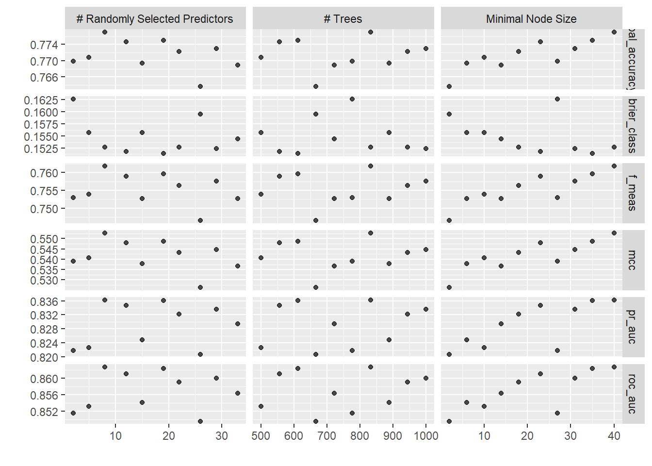
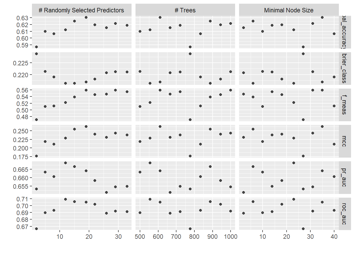
Now, that we have fitted the model with the hyperparameter configurations, we can retrieve the results of the performances of the fitted models. This can be done using collect_metrics() to get them in tabular format or plot the results using autoplot().
Let’s extract the best hyperparameter configuration through select_best(), update the workflow using finalize_workflow() and fit it to the whole training dataset with fit(). We have used here the Mathews Correlation Coefficient as a metric for hyperparameter selection. Choose the metric that fits best with the goal of your model.
Now, let’s repeat the process for using the SpaceTime_CV folds. As you can see below, you don’t have to repeat all the process but just provide the tuning function with a different CV folds object.
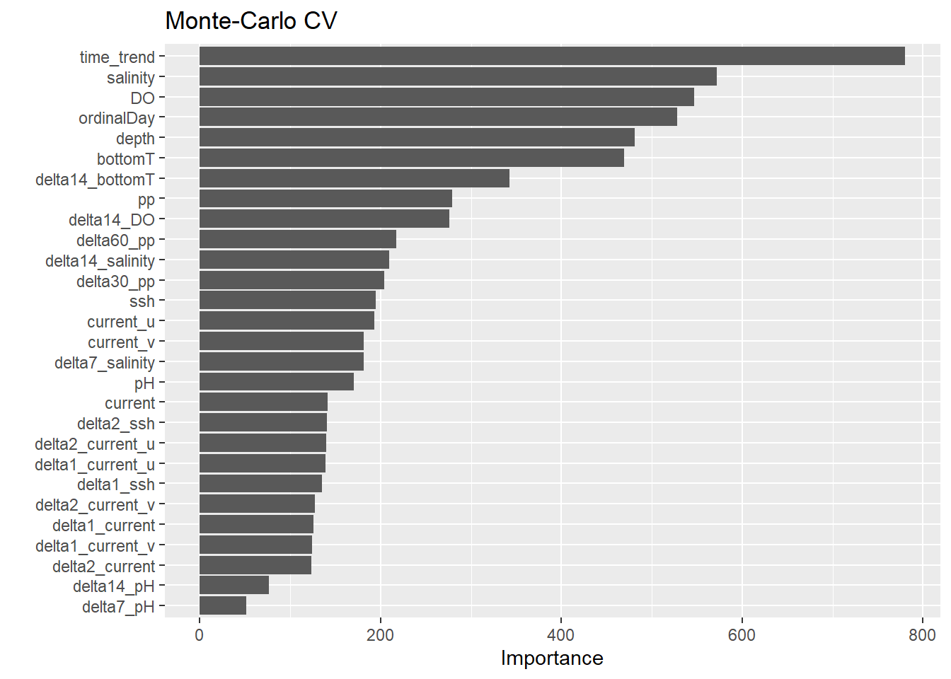
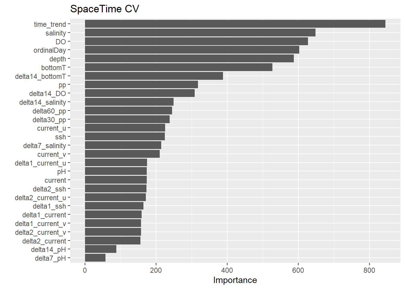
You can further simplify your model by removing factors that have very small contribution to the model fitting. Remember that how we specified importance="impurity" in the our random forest parsnip model. We can use this to rank the predictors based on their Importance Values. We can use the package vip. You can pass the trained workflow to the function vip() to plot the ranks or vi() to get the tabular results.
To simplify the model without compromising performance, feature (predictor) selection can be employed. This involves identifying the optimal set of predictors to retain. Several methods are available for this purpose, including forward selection, backward elimination, and recursive feature elimination (RFE). In this workflow, we will use RFE. This method works by recursively removing the least important features and building the model iteratively to evaluate the performance at each step. By doing so, RFE ensures that only the most essential predictors are retained, balancing model simplicity and accuracy.
The first step in recursive feature elimination (RFE) is to choose a metric, as it will guide the elimination process. Here, we will use the Area Under the Precision-Recall Curve (PR AUC), which we have already utilized previously. A PR AUC value close to 1 indicates a well-performing model. Next, define a vector to store the names of the predictors. Additionally, create a tibble to record the tuning results for each iteration of the elimination process. It’s also important to set baseline threshold values for the metric. Since the goal is to maximize PR AUC toward a value of 1, we will initialize these thresholds on the opposite end of the spectrum, at 0. Moreover, we will be expanding the grid to more values using latin_hypercube sampling. This divides the parameter space into equal-sized intervals and sample points such that each parameter dimension is evenly represented.
During each iteration of recursive feature elimination (RFE), predictors will be removed incrementally until model performance no longer improves. The following steps outline the process:
Updating the Recipe, Workflow, and Grid: For every iteration, the recipe and workflow must be updated with new template data to reflect the current set of predictors. The grid should also be updated because mtry depends on the number of predictors.
Model Fitting: The model fitting procedure is conducted in the same manner as before, with results of the tuning process stored in the predefined tibble tune_results.
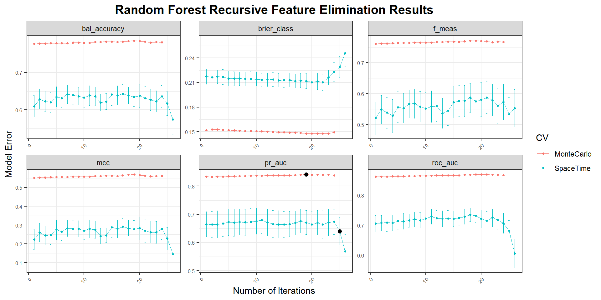
Visualizing Performance Evolution: To track the progression of model performance across iterations, a plot can be generated to visualize the metric’s evolution.
Performance Evaluation: At the end of each iteration, the performance of the current model is evaluated and compared to the performance of the previous iteration. If the metric value starts to deteriorate, the recursive elimination loop is terminated. However, if the metric value exceeds the threshold or remains within 1 standard error of the performance from the previous iteration, the elimination process continues.
Threshold and Template Data Update: If the current model’s performance shows significant improvement over the previous iteration, the threshold values are updated to reflect the current metric values. Moreover, the template data should be updated based on the current set of predictors.
When plotting the tuning results for both Monte Carlo and SpaceTime cross-validation strategies, the SpaceTime CV approach yielded weaker model performances. The black point indicates the optimal set of predictors using one standard error rule.
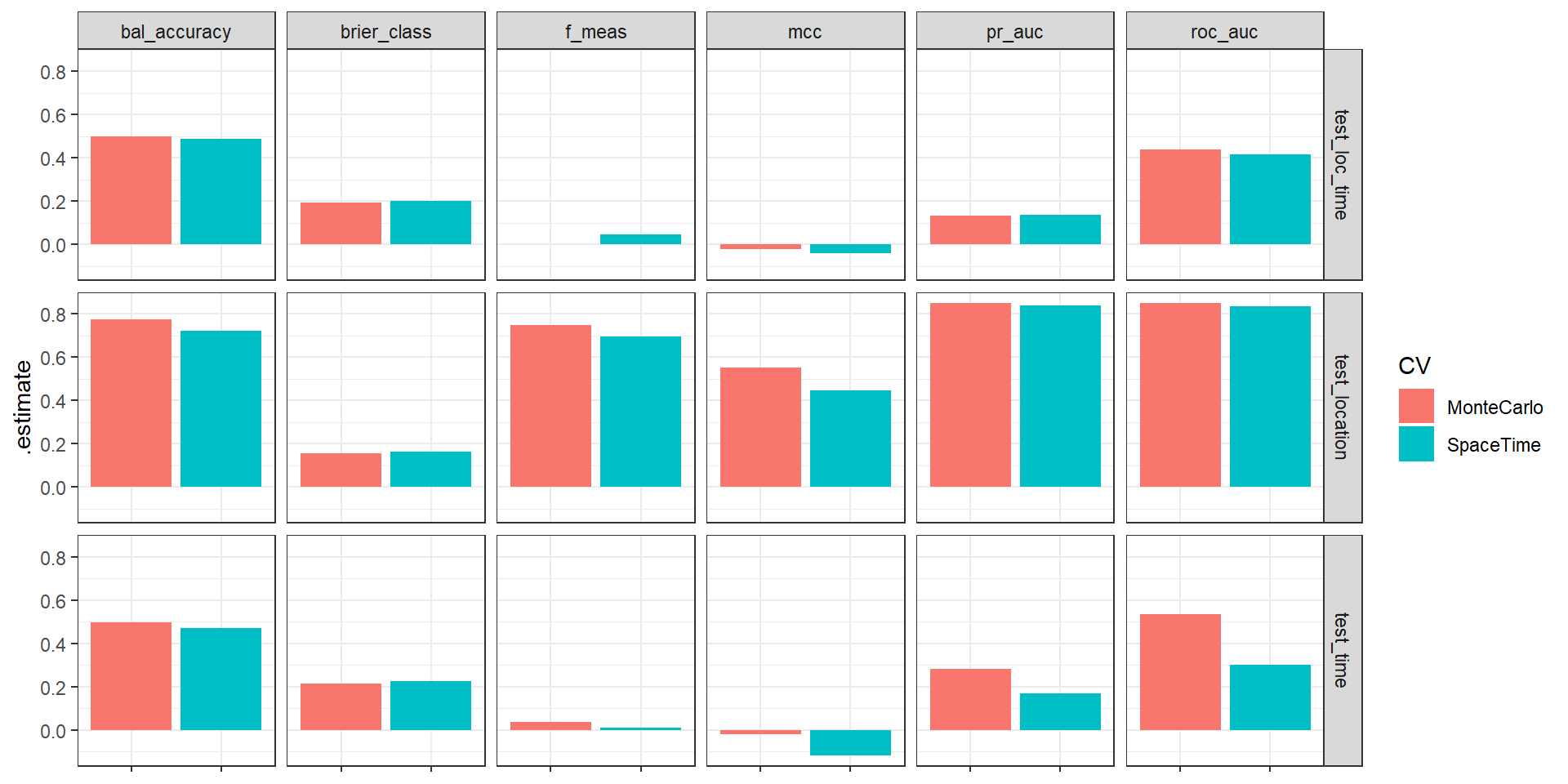
Finalize the workflow using the optimal hyperparameter configuration selected by Monte Carlo cross-validation. Repeat the process with SpaceTime cross-validation.
After selecting the best model, you can save a simplified version of the workflow to reduce its size. The butcher package can be used to strip the workflow object of unnecessary components, such as the input training data. Additionally, it is considered good practice to create metadata for the trained workflow, documenting key information such as the selected model, hyperparameters, and performance metrics.
library(butcher) workflow_butcher <-butcher(final_workflow_MCCV)error <- results %>%filter(CV=="MonteCarlo") %>%rename(test_type = data_split) %>%mutate(.metric_info =case_when(.metric=="f_meas"~"F1 Score", .metric=="mcc"~"Matthews correlation coefficient", .metric=="bal_accuracy"~"Balanced accuracy", .metric=="brier_class"~"Brier score for classification models", .metric=="roc_auc"~"Area under the receiver operator curve", .metric=="pr_auc"~"Area under the precision recall curve",TRUE~"other"),test_type_info =case_when(test_type=="test_location"~"The model's extrapolation performance was assessed on new locations, but within the training data's time range", test_type=="test_time"~"The model's extrapolation performance was evaluated on future data, but within the training data's spatial range", test_type=="test_loc_time"~"The model's extrapolation power was tested in space and time.",TRUE~"other"),Predictors =list(MCCV_predictors)) metadata <-list(contact ="Clyde Blanco",institute ="Instituut voor Landbouw-, Visserij- en Voedingsonderzoek (ILVO)",model ="Random Forest",library ="tidymodels 1.2.0",creation_date =Sys.Date(),model_metrics = error, training_data ="Catch data of common sole (Solea solea) from ILVO's databases (SmartFish and VISTools) coupled with CMEMS ocean physics and biogeochemistry products.",notes ="Hyperparameter tuning and recursive feature selection were employed during the training process.")workflow_with_metadata <-list(workflow = workflow_butcher,metadata = metadata)saveRDS(workflow_with_metadata, "workflow_with_metadata.rds")