# Dependencies ------------------------------------------------------------

# install.packages(c("terra","dplyr","ncdf4","shiny","shinyWidgets","bslib",
#                    "leaflet","leafem","scico","sf"))

library(terra)
library(dplyr)
library(ncdf4)
library(shiny)
library(shinyWidgets)
library(bslib)
library(leaflet)
library(leafem)
library(scico)
library(sf)

# The script behind the Shiny app has 3 groups of codes. The first group of codes
# will load the predictions to be visualized and the metadata of these predictions.
# The second group designs the User Interface of the app and the contents dynamically
# change with any user input. The third group is the server where any user inputs
# activities are processed and cause a change in the UI.


# Load Rasters ----------------------------

nc_files <- list.files(path = "./../Models/Predictions",                        # Load NetCDF file paths
                       pattern='.nc$',
                       all.files=TRUE,
                       full.names=TRUE)

land <- vect("./../Data/Raw/Polygons/Europe.shp")                               # Load Europe land polygon

mask <- vect("./../Data/Raw/Polygons/mask.shp")                                 # Load masking polygon as SpatVector

predictions <- rast(nc_files)                                                   # Load NetCDF files as SpatRasters
predictions <- terra::mask(predictions,land, inverse=TRUE)                      # Remove raster cells that overlaps with land

names(predictions) <- substring(names(predictions),1,3)                         # Rename SpatRaster layers to FAO codes (i.e., SOL and PLE)

max_values <- numeric()

for(i in unique(names(predictions))){
  max_values <- c(max_values,
                  max(values(predictions[[names(predictions)==i]]),na.rm=TRUE))
}
names(max_values) <- unique(names(predictions))

masked_pred <- mask(predictions,mask)                                           # Keep raster cells within the masking polygon. This will only show predictions where validation data is present.

Dates <- unique(terra::time(predictions))                                       # extract Dates to be used in the Date slider in the UI

mask <- st_read("./../Data/Raw/Polygons/mask.shp")                              # Reload masking polygon as sf

raster_list <- vector(mode="list", length = length(unique(names(predictions)))) # Create a list that will store the prediction raster files
names(raster_list) <- unique(names(predictions))                                # Name the elements of the list with FAO codes

for(i in unique(names(predictions))){                                           # This for loop will extract a raster from the SpatRaster and convert it to an RasterLayer and store it in the raster_list

  mask_list <- vector(mode="list", length=2)                                    # Create a list of 2 elements - the whole prediction area and the cropped raster
  names(mask_list) <- c("mask","whole_area")

  for(j in names(mask_list)){
    raster <- if(j=="mask") masked_pred else predictions                        # Choose which SpatRaster to process depending on current middle loop iteration

    dates_list <- vector(mode="list", length=length(Dates))                     # Create a list that will contain the daily predictions RasterLayer
    names(dates_list) <- Dates

    for(k in 1:length(Dates)){
      subRaster <- raster[[names(raster)==i]]                                   # Subset raster based on the current species in the outer loop iteration
      subRaster <- subRaster[[terra::time(subRaster)==as.POSIXct(Dates[k])]]    # Subset raster based on the current Date in the inner loop iteration

      dates_list[[k]] <- raster::raster(terra::project(subRaster,"EPSG:3857"))  # Project raster to EPSG:3857 and convert to RasterLayer. Leaflet can only visualize RasterLayer and not SpatRaster.
    }

    mask_list[[j]] <- dates_list
  }

  raster_list[[i]] <- mask_list
}

rm(mask_list,dates_list) # Clean up to free up some memory8.2 Interactive Visualisation
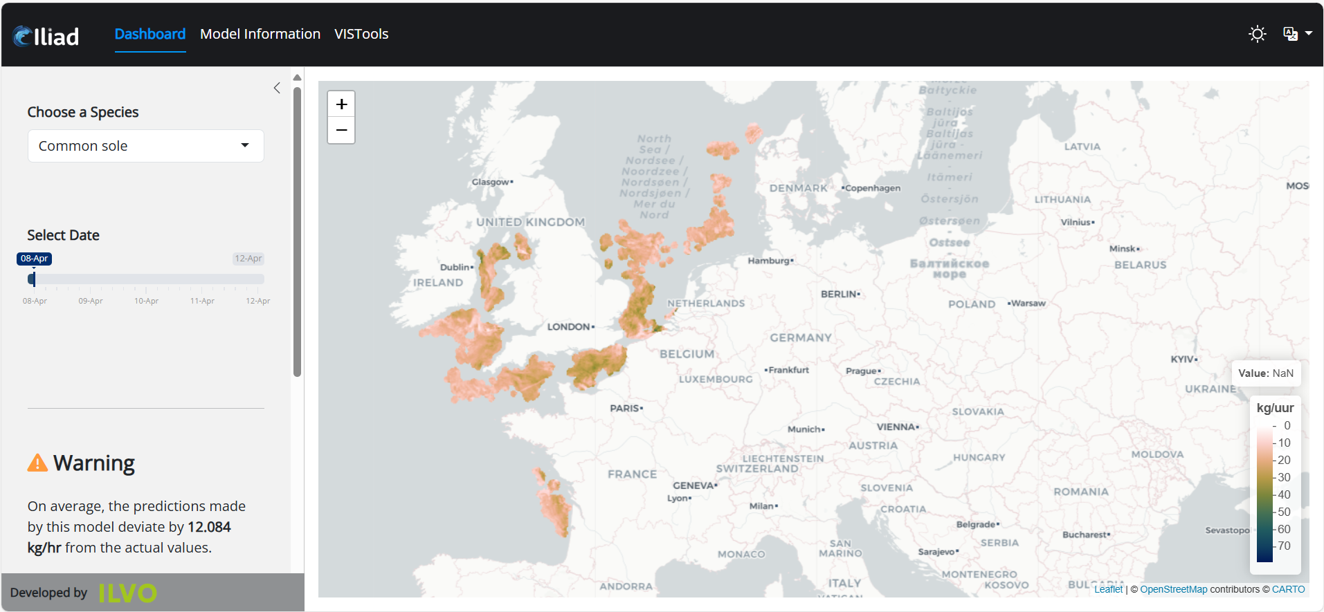
The Catch Predictions Dashboard (Figure 1) is build using Shiny for R. Shiny is an R package that makes it easy to develop interactive web applications (apps) straight from R. The Catch Predictions Dashboard is a Shiny app contained in a single R-script. This script comprises of three key components:
- the user interface (
ui) - the
serverfunction - a call to the
shinyAppfunction
The ui defines the layout and appearance of the app, the server function contains the logic to build the app’s outputs based on user inputs, and the shinyApp function brings the ui and server together to create the app. In the following sections we will go through all components of the Shiny app’s code and explain what each does within the Catch Predictions Dashboard. Basic knowledge on Shiny is required and can be found on the developer’s website.
First things first
At the beginning of the Shiny script the NetCDF files containing the model predictions (see subsection 8.1) are loaded and processed to allow displaying catch predictions for common sole (Solea solea) or European plaice (Pleuronectes platessa) on the map, and extraction of metadata that is used for text (see next paragraph) and other components of the app. The code for importing the NetCDF files is placed outside the ui and server function as these will be loaded only once during the start-up of the app and not anymore during processes performed within the server. Loading and processing NetCDF files only once at start-up increases computational efficiency of the Shiny App.
All metadata and text that should be displayed in the user interface is created in Dutch and English in a translation directory named translations. Depending on the input in the user interface ui a selection of text objects is made from the translations list in the appropriate language based on the logic defined in the server of the app. The translation directory translations is build outside the ui and server. Such placing of this code block allows for a cleaner server logic code later on.
# Create Translation Directory ----------------------------

nc_info <- vector(mode="list",length=2)

for(i in 1:length(nc_files)){                                                   # This for loop will create a list that will contain the model metadata both in English and Dutch

  nc <- nc_open(nc_files[i])                                                    # Open NetCDF file to extract metadata

  source <- ncatt_get(nc,0)$source                                              # ML algorithm used in model training
  library <- ncatt_get(nc,0)$library                                            # R package used in ML model training
  comment_en <- ncatt_get(nc,0)$comment                                         # Extra information on the training data and fitting process
  contact <- ncatt_get(nc,0)$contact                                            # Modeller
  eval_date = gsub("evaluated on ","",                                          # Date of model evaluation
                   regmatches(comment_en,
                              regexpr("evaluated on (\\d{2}-[A-Za-z]{3}-\\d{4})",
                                      comment_en)))

  # The following codes extracts more information from the metadata and create
  # different language versions. These texts will be used in the UI depending on
  # the selected species and language.

  if(grepl("plaice",comment_en)){
    Species = "PLE"
    sp_name = "schol (Pleuronectes platessa)"
    log_trans = "De vangstwaarden werden getransformeerd met de formule log(CPUE+0,00001)."
    error = gsub("hr","uur",
                 regmatches(comment_en,
                            regexpr("\\d+\\.\\d+\\s*kg/hr",comment_en)))

  } else {
    Species = "SOL"
    sp_name = "tong (Solea solea)"
    log_trans = ""
    error = gsub("hr","uur",
                 regmatches(comment_en,
                            regexpr("\\d+\\.\\d+\\s*kg/hr",comment_en)))
  }

  comment_nl <- paste0("De vangstgegevens voor de ",sp_name," werden opgehaald uit de ILVO-databases (SmartFish en VISTools)",
                       " en zijn gekoppeld aan oceaanfysica- en biogeochemische gegevens van Marine Copernicus en statische zeebodemvariabelen van EMODnet.",
                       "Tijdens het trainingsproces werden hyperparameters getuned en recursieve featureselectie toegepast om het model te optimaliseren. ",
                       log_trans, " De extrapolatieprestaties van het model werden geëvalueerd met gegevens uit 2024 (07-Jan-2024 to 07-Jun-2024)",
                       ", wat resulteert in een root mean square error (RMSE) van ",
                       error, ". De modelprestaties werden geëvalueerd op ",eval_date,".")

  if(grepl("and decision trees as base learners",source)){
    source_nl <- sub("and decision trees as base learners","met decision trees als basisleerders",source)

    if(grepl("with Tweedie regression",source_nl)){
      source_nl <- sub("with Tweedie regression","en Tweedie-regressie",source_nl)
    }
  }


  nc_info[[i]] <- list(
    model_info_en =  HTML(paste0("The Machine Learning (ML) algorithm used to train the data is ",
                                 source,", using the R package ", library, ". <br><br>",
                                 gsub("\\((\\b[A-Z][a-z]+\\s[a-z]+\\b)\\)","(<i>\\1</i>)",comment_en),
                                 "<br><br>To know more about the model training process, contact ",
                                 contact,"or visit this <a href='https://vistools.quarto.pub/iliad-pilot-documentation/sections/guide/07_01_fish_suit.html' target='blank'>documentation</a>.")),
    dash_info_en = HTML(paste0("On average, the predictions made by this model deviate by ","<strong>",
                               regmatches(comment_en,regexpr("\\d+\\.\\d+\\s*kg/hr",comment_en)),
                               "</strong>"," from the actual values.")),
    model_info_nl =  HTML(paste0("Het Machine Learning (ML) algoritme dat is gebruikt om de gegevens te trainen is, ",
                                 source_nl," met behulp van de R-package ", library, ". <br><br>",
                                 gsub("\\((\\b[A-Z][a-z]+\\s[a-z]+\\b)\\)","(<i>\\1</i>)",comment_nl),
                                 "<br><br>Voor meer informatie over het modeltrainingsproces kunt u contact opnemen met ",
                                 contact," of ga naar deze <a href='https://vistools.quarto.pub/iliad-pilot-documentation/sections/guide/07_01_fish_suit.html' target='blank'>documentatie</a>."
    )),
    dash_info_nl = HTML(paste0("Gemiddeld wijken de voorspellingen die door dit model gemaakt worden ","<strong>",
                               gsub("hr","uur",
                                    regmatches(comment_en,regexpr("\\d+\\.\\d+\\s*kg/hr",comment_en))),
                               "</strong>"," af van de werkelijke waarden."))
  )
  names(nc_info)[i] <- Species

  nc_close(nc)

}

# The following codes will create a directory of texts both in English and Dutch.
# Depending on the selected languages, the UI texts will dynamically change. Codes
# wrapped in <>...</> are HTML codes and these will be rendered as HTML tags in
# the UI instead of just being plain texts.

translations <- list(
  en = list(
    choose_species = "Choose a Species",
    species_mapping = c("Common sole" = "SOL", "European plaice" = "PLE"),
    choose_date = "Select Date",
    warning_lab = HTML('<i class="fa-solid fa-triangle-exclamation" style="color: #ff9b3d;"></i> <strong>Warning</strong>'),
    modal_msg = "The catch values you see here are based on predictions made by the models and, as such,
          come with inherent uncertainty and potential error. These values do not perfectly reflect
          reality and should not be treated as absolute truths. They serve as a guide, providing useful insights,
          but it is important to approach them with caution. Decisions should be made considering these predictions
          along with other relevant factors, such as your knowledge of the fisheries, local conditions,
          and practical experience. Recognizing the limitations of the model, these insights should be used as one of several inputs in the decision-making process.",
    dash_info = list(
      PLE = nc_info[["PLE"]][["dash_info_en"]],
      SOL = nc_info[["SOL"]][["dash_info_en"]]
    ),
    model_info = list(
      PLE = nc_info[["PLE"]][["model_info_en"]],
      SOL = nc_info[["SOL"]][["model_info_en"]]
    ),
    dash_about = "The underlying model was trained on data from a specific set of catch locations.
          The default map shows predictions within a 10 km radius of the training data points.
          Predictions for areas beyond this range may be unreliable due to lack of validation.
          Use the model only in locations where applicability has been confirmed,
          and exercise caution when applying it to new areas. To view predictions for the entire region,
          please enable the option below.",
    dash_show = HTML("Show Entire Prediction Area"),
    tab_title = "Model Information",
    page_model_title = "Description",
    leaflet_unit = "kg/hr",
    map_warning = "<div style='background: #fff3cd; padding: 12px; border-radius: 5px; font-size: 18px; color: #856404;'><strong>Note: </strong>Predictions in areas enclosed by the black line are validated.</div>"

  ),
  nl = list(
    choose_species = "Kies een Soort",
    species_mapping = c("Tong" = "SOL", "Schol" = "PLE"),
    choose_date = "Selecteer Datum",
    warning_lab = HTML('<i class="fa-solid fa-triangle-exclamation" style="color: #ff9b3d;"></i> <strong>Waarschuwing</strong>'),
    modal_msg = "De vangstwaarden die je hier ziet, zijn gebaseerd op voorspellingen van de modellen en brengen daardoor inherente onzekerheid en
          mogelijke fouten met zich mee. Deze waarden weerspiegelen niet volledig de werkelijkheid en moeten niet worden behandeld als
          absolute waarheden. Ze dienen als een gids en bieden nuttige inzichten, maar het is belangrijk om ze met voorzichtigheid
          te benaderen. Beslissingen moeten worden genomen door deze voorspellingen te overwegen, samen met andere relevante factoren,
          zoals jouw kennis van de visserij, lokale omstandigheden en praktische ervaring. Het model heeft zijn beperkingen en moet
          gebruikt worden als één van de verschillende hulpmiddellen in je het besluitvormingsproces.",
    dash_info = list(
      PLE = nc_info[["PLE"]][["dash_info_nl"]],
      SOL = nc_info[["SOL"]][["dash_info_nl"]]
    ),
    model_info = list(
      PLE = nc_info[["PLE"]][["model_info_nl"]],
      SOL = nc_info[["SOL"]][["model_info_nl"]]
    ),
    dash_about =  "Het onderliggende model is getraind op gegevens van een specifieke lijst van vangstlocaties.
      De standaardkaart toont voorspellingen die binnen een straal van 10 km liggen van de trainingsdatapunten.
      Voorspellingen voor de gebieden buiten deze straal zijn onbetrouwbaar door het gebrek aan validatie.
      Gebruik het model alleen op de locaties waar de validatie en toepasbaarheid bevestigd is,
      en wees voorzichtig wanneer het op een nieuw gebied toegepast wordt. Om voorspellingen voor de gehele regio te bekijken,
      zet de optie hieronder aan.",
    dash_show = HTML("Toon Het Hele <br>Voorspellingsgebied"),
    tab_title = "Modelinformatie",
    page_model_title = "Beschrijving",
    leaflet_unit = "kg/uur",
    map_warning = "<div style='background: #fff3cd; padding: 12px; border-radius: 5px; font-size: 18px; color: #856404;'><strong>Opmerking: </strong>Voorspellingen in gebieden omgeven door de zwarte lijn zijn gevalideerd.</div>"
  )
)
User Interface (UI)

The backbone of the app is defined as the user interface ui and is a top level navigation bar (page_navbar) that is used to toggle a set of panels (i.e. nav_panel() elements contained within the page_navbar function; Figure 2). Some of the layout of the app is generated through HTML tags. For instance, tags$link defines the relationship between the shiny app script and an external style sheet that allows the use of Font Awesome. The app is available in Dark and Light mode (hit the ![]() button in the upper right corner) and in Dutch and English (choose from the drop-down menu
button in the upper right corner) and in Dutch and English (choose from the drop-down menu ![]() in the upper-right corner).
in the upper-right corner).
# Define the UI ----------------------------
ui <- page_navbar(                                                              # This will render a User Interface with a sidebar navigation and 3 tabs, light-dark switch, and language switch

  # import the CSS to use Bootstrap icons
  tags$head(                                                                    # The tags object in shiny is a list of 100+ simple functions that create HTML tags, some of which are used here to layout the Shiny App
    tags$link(rel = "stylesheet",
              href = "https://cdn.jsdelivr.net/npm/bootstrap-icons/font/bootstrap-icons.css"),

    # import the CSS to use Font Awesome
    tags$link(rel = "stylesheet",
              href = "https://cdnjs.cloudflare.com/ajax/libs/font-awesome/6.4.2/css/all.min.css"),

    # CSS codes to customize the UI
    tags$style(
      HTML("
        .modal-dialog {
          position: fixed;
          top: 50% !important;
          left: 50% !important;
          transform: translate(-50%, -50%) !important;
          margin: 0 !important;
        }
        .modal-content {
          background-color: #fff3cd;
          border: 2px solid #856404;
          border-radius: 15px;
          padding: 30px;
          box-shadow: 0px 4px 15px rgba(0, 0, 0, 0.1);
        }
        .modal-title {
          font-size: 30px;
          font-weight: bold;
          color: #856404;
        }
        .modal-body {
          font-size: 18px;
          color: #6c757d;
          padding: 20px 0;
        }
        .modal-icon {
          font-size: 30px;
          color: #856404;
          text-align: center;
          margin-bottom: 20px;
        }
        .dark-mode select {
        background-color: #333;  /* Dark background */
        color: white;  /* Light text */
        }
      ")
    )
  ),

  title = tags$a(                                                               # The Iliad logo that links to the iliad Marketplace website
    href = "https://ocean-twin.eu/marketplace",
    target = "_blank",
    tags$img(
      src = "https://vistools.quarto.pub/iliad-pilot-documentation/images/iliad_logo.png",
      height = "25px",
      style = "padding: 0; margin-right: 10px; "
    )
  ),
  bg =  "#1A1B1E",                                                              # The background color of the top level navigation bar

  window_title = "Catch Predictions",

  theme = bs_theme(                                                             # The general theme of the Shiny App
    version = 5,
    bootswatch = "flatly",
    primary = "#0197F6",
    base_font = font_google("Open Sans"),
    nav_font = font_google("Roboto")
  ),

  # First tab
  nav_panel(                                                                    # The first tab showing the Catch Predictions Dashboard
    tags$head(
      tags$style(HTML("
      .shiny-input-container label {
        font-weight: bold;
      }
    "))
    ),
    title = "Dashboard",
    layout_sidebar(
      sidebar = sidebar(                                                        # A floating sidebar displayed on the left-hand side of the page which allows the user to adjust features shown on the map
        padding = c(40,30,0,30),
        width = "350px",
        selectInput(                                                            # drop down menu to choose the species that is to be displayed on the map
          inputId = "species",
          label = textOutput("dash_sp_label"),
          width = "280px",
          choices = c("Tong" = "SOL", "Schol" = "PLE")),
        br(),
        chooseSliderSkin("Flat", color="#002F70"),                              # Slider to select the date for which predictions are to be displayed on the map
        sliderInput(inputId = "date",
                    label = textOutput("dash_date_label"),
                    min = as.Date(min(Dates)),
                    max = as.Date(max(Dates)),
                    value = as.Date(min(Dates)),
                    step = 1,
                    width = "280px",
                    timeFormat = "%d-%b"),
        br(),
        br(),
        br(),
        hr(),
        p(h4(
          uiOutput("dash_warning_label"), inline=TRUE),                         # Text describing the estimated mean deviation of the predictions versus reality
          span(htmlOutput("overlay_text"))),

        p(textOutput("dash_about_label")),                                      # Text describing how to use displayed predictions and best deal with uncertainties
        materialSwitch(inputId = "whole_area",                                  # switch to turn off (or back on) the mask over the areas with low data availability
                       label = htmlOutput("dash_showArea_label"),
                       status="danger",
                       right=T, inline=T),
        br(),
        br(),
        div(                                                                    # footnote on developer (ILVO) with custom styling and clickable logo which redirects to developers website
          style = "position: fixed; bottom: 0; left: 0; width: 350px; padding: 10px; text-align: left; background-color: #8F9193;",

          tags$span("Developed by", style = "font-size: 14px; font-weight: bold; margin-top: 5px;"),

          tags$a(
            href = "https://ilvo.vlaanderen.be/nl/",
            target = "_blank",
            tags$img(src = "https://vistools.quarto.pub/iliad-pilot-documentation/images/ILVO_logo.png",
                     width = "70px",
                     style = "display: inline-block; vertical-align: middle; margin-left: 10px;")
          )

        )
      ),
      leafletOutput("map", width = "100%", height = "100%"),                    # a leaflet map is set as main content within layout_sidebar()
    )
  ),

  # Second tab
  nav_panel(                                                                    # Second tab with information text on model development
    title = textOutput("nav_info_label"),                                       # The tab name is either "Modelinformatie" or "Model Information" depending on the language
    tags$style(HTML("
    .styled-text {
      margin: 20px 30px 10px 30px;
      padding: 15px;
      background-color: #f9f9f9;
      border-radius: 10px;
      box-shadow: 0 4px 8px rgba(0, 0, 0, 0.1);
      color: #333;
      }
    .styled-text h3 {
      font-size: 2em;
      color:  #1940c3;
      font-weight: bold;
      }
    .styled-text p {
      font-size: 1.2em;
      line-height: 1.5;
      }
    ")),
    div(class="styled-text",
        h3(textOutput("info_title_label")),                                     # The tab title is either "Beschrijving" or "Description" depending on the language
        p(span(htmlOutput("layer_description")))                                # Information on model development, either in Dutch or English
    )
  ),

  nav_item(a(href = "https://vistools.be", "VISTools")                          #  Third tab which links to VISTools Analyses dashboard
  ),

  nav_spacer(),
  nav_item(input_dark_mode(id = "mode", mode="light")),                         # A button that toggles between dark and light modes on the right-hand side of the top level navigation bar
  nav_menu(                                                                     # A drop down menu to select the language on the right-hand side of the top level navigation bar
    HTML('<i class="bi bi-translate"></i>'),
    nav_item(actionLink("lang_nl","NL")),
    nav_item(actionLink("lang_en","EN")),
    align="right"
  )
)
Server logic
The server function contains the logic to build the app’s outputs based on user inputs generated in the user interface ui. The Catch Predictions Dashboard server controls what text is displayed in what language and what data is shown on the map based on the values that a user selects in the app.
English versus Dutch language through reactiveVal() and a Translation Directory
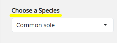
All text in the app is either displayed in Dutch or English depending on which list item (either "nl" or "en") is extracted from the translation directory translations. In which language the text is to be extracted is determined by the reactive value (reactiveVal()) named lang which is created in the server logic and is implemented as follows: translations[[lang()]]. The resulting list is then further subsetted in order to place the appropriate text blocks at the appropriate locations in the user interface. An example is the label dash_sp_label (Figure 3). This label is contained within the output object and relates to a textOutput() function in the user interface ui that generates the label of a drop-down menu to choose the displayed species on the map. The associated text of the label is contained within translations[[lang()]]$choose_species.
To a lesser extent, the reactive value lang is also used in if else statements and within observe() and observeEvent() functions throughout the server logic.
# Define server logic ----------------------------
server <- function(input, output, session) {

  lang <- reactiveVal("nl")                                                     # Set initial language value to "nl". Depending on the given input in the user interface's drop down menu this can change to "en"
  sp <- reactiveVal(NULL)
  date <- reactiveVal(NULL)
  area <- reactiveVal(NULL)

  observeEvent(input$lang_en, {                                                 # if user changes the language in the drop-down menu to English change the reactive value lang accordingly
    lang("en")
  })

  observeEvent(input$lang_nl, {                                                 # Change everything back to Dutch if user switches the language back to Dutch
    lang("nl")
  })

  observe({                                                                     # Show the disclaimer in the appropriate language at page entry and when the language is adjusted
    if(lang() %in% c("nl","en")){
      showModal(
        modalDialog(
          title = tags$div(
            icon("exclamation-triangle", class = "modal-icon"),
            "Disclaimer"
          ),
          easyClose = TRUE,
          translations[[lang()]]$modal_msg
        )
      )
    }

    updateSelectInput(session, "species", choices = translations[[lang()]][["species_mapping"]])
  })                                                                            #

  output$dash_sp_label <- renderText({translations[[lang()]]$choose_species})   # Display the text label for the drop-down menu from the sidebar of the first panel either in Dutch or English
  output$dash_date_label <- renderText({translations[[lang()]]$choose_date})    # Display the text label for the slider from the sidebar of the first panel either in Dutch or English
  output$dash_warning_label <- renderUI({translations[[lang()]]$warning_lab})   # Display the text label on estimated mean deviation of the predictions versus reality from the sidebar of the first panel either in Dutch or English
  output$overlay_text <- renderUI({translations[[lang()]][["dash_info"]][[input$species]]})
  output$dash_about_label <- renderText({translations[[lang()]]$dash_about})    # Display the text on how to use displayed predictions from the sidebar of the first panel either in Dutch or English
  output$dash_showArea_label <- renderUI({translations[[lang()]]$dash_show})    # Display the text label for the switch to turn off (or back on) the mask on the areas with low data availability either in Dutch or English
  output$nav_info_label <- renderText({translations[[lang()]]$tab_title})       # Display the name of the second tab either in Dutch or English
  output$info_title_label <- renderText({translations[[lang()]]$page_model_title})  # Display the main title in the second tab either in Dutch or English
  output$layer_description <- renderUI({translations[[lang()]][["model_info"]][[input$species]]})  # Information on model development that is displayed in tab two, either in Dutch or English, is dependent on the chosen species in tab one
Building the map
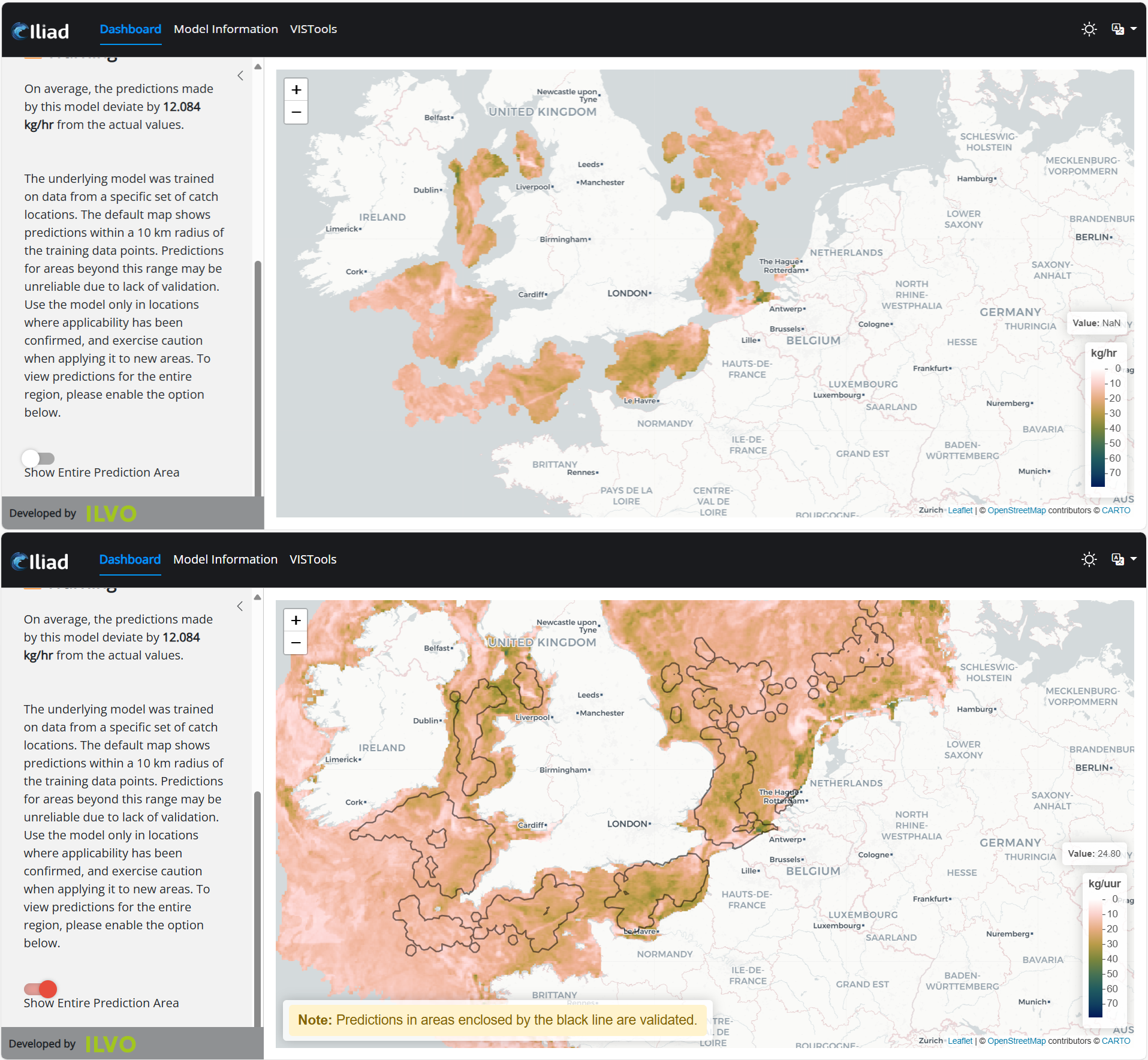
A map is generated by layering geographic location labels and a catch prediction raster on top of a base map which is either dark or light depending on the mode selected by the user. The catch prediction raster is pulled from a raster_list build out of the netCDF files loaded upon start-up of the app. Which raster is pulled is determined through the reactive expression raster and is based on the species chosen from a drop-down menu in the sidebar of the first tab and the date selected on a slider. A switch in the user interface determines whether a masked raster is shown with predictions for only the validated areas or the whole area (Figure 4).
  observe({                                                                     # set the input parameters to generate the appropriate map
    sp(input$species)
    date(as.character(input$date))
    if(input$whole_area) area("whole_area") else area("mask")
  })

  raster <- reactive({                                                          # create reactive expression that selects the appropriate raster from the raster list based on the species, area and date user input
    raster_list[[sp()]][[area()]][[date()]]
  })

  max_value <- reactive({                                                       # create reactive expression for the maximum predicted value of the selected raster layer to enable setting the color scale
    max_values[sp()]
  })

  pal <- reactive({                                                             # create reactive expression to set the color scale of the map
    colorNumeric(
      palette = scico(n = 10, palette = "batlowW", direction = -1),
      domain = c(0, max_value()), na.color = "transparent"
    )
  })

  base_map <- reactive({                                                        # create reactive expression to switch between dark and light base maps depending on the input of the dark and light mode switch
    if (input$mode == "light") "CartoDB.PositronNoLabels" else "CartoDB.DarkMatterNoLabels"
  })

  base_map_label <- reactive({                                                  # create reactive expression to switch between dark and light base map labels depending on the input of the dark and light mode switch
    if (input$mode == "light") "CartoDB.PositronOnlyLabels" else "CartoDB.DarkMatterOnlyLabels"
  })

  output$map <- renderLeaflet({                                                 #  Create the map

    leaflet() %>%                                                               # Set the location and zoom level for the base map in the first tab; the layers are added in the following lines of code
      setView(lng = 1.5, lat = 51.5, zoom = 6)

  })

  observeEvent(input$mode,{                                                     # If switching between light and dark mode, adjust layers of map accordingly using the reactive values created before
    leafletProxy("map") %>%                                                     # Creates a map-like object that can be used to customize and control a map that has already been rendered
      clearTiles() %>%
      clearImages() %>%
      clearShapes() %>%
      clearControls() %>%
      addProviderTiles(base_map(), layerId = "BaseMap") %>%                     # add the base map (either light or dark)
      addRasterImage(raster(), colors = pal(), opacity = 1, group = "Value", project = TRUE, layerId="Raster") %>%    # add the appropriate raster layer that was selected based on species, area and date
      addProviderTiles(base_map_label(), layerId = "MapLabels") %>%             # add the labels on top of the selected raster layer
      addLegend("bottomright", title = translations[[lang()]]$leaflet_unit, values = c(0, max_value()), pal = pal(), opacity = 1) %>%   # add legend in the appropriate language
      leafem::addImageQuery(x = raster(), project = TRUE, group = "Value", prefix = "", position = "bottomright", digits = 2)   # Add image query functionality in which value is shown when hoovering the pointer over the map

    if(input$whole_area){                                                       # Depending on the input of the area switch add polygon layer indicating the areas that are verified with VISTools data
      leafletProxy("map") %>%
        addPolygons(data = mask, layerId = "AreaCover",
                    color = "black", weight = 2, fill = FALSE) %>%
        addControl(html = translations[[lang()]][["map_warning"]],
                   position = "bottomleft", layerId = "Warning")                # If no masking layer is present add a warning message in the bottomleft corner of the map
    }
  })

  observeEvent(list(input$species,input$date,input$whole_area),{                # If the user changes the species, date or area, adjust layers of map accordingly using the reactive values created before

    leafletProxy("map") %>%
      removeImage(layerId = "Raster") %>%
      removeShape(layerId = "AreaCover") %>%
      removeTiles(layerId = "MapLabels") %>%
      clearControls() %>%
      addRasterImage(raster(), colors = pal(), opacity = 1, group = "Value", project = TRUE, layerId="Raster") %>%
      addProviderTiles(base_map_label(), layerId = "MapLabels") %>%
      addLegend("bottomright", title = translations[[lang()]]$leaflet_unit, values = c(0, max_value()), pal = pal(), opacity = 1) %>%
      leafem::addImageQuery(x = raster(), project = TRUE, group = "Value", prefix = "", position = "bottomright", digits = 2)

    if(input$whole_area){
      leafletProxy("map") %>%
        addPolygons(data = mask, layerId = "AreaCover",
                    color = "black", weight = 2, fill = FALSE) %>%
        addControl(html = translations[[lang()]][["map_warning"]],
                   position = "bottomleft", layerId = "Warning")
    }
  })

  observeEvent(lang(),{                                                         # If the language changes, adjust the warning text in the bottom left corner of the map accordingly
    if(input$whole_area){
      leafletProxy("map") %>%
        removeControl(layerId = "Warning") %>%
        addControl(html = translations[[lang()]][["map_warning"]],
                   position = "bottomleft", layerId = "Warning")
    }
  })
}
Run the app!
Now we are only one line of code away of making the magic happen, that is, making the app work! Time to see where we can expect to find high catches of the selected flatfish!
shinyApp(ui = ui, server = server)